If the determinant of a matrix is zero, then its inverse does not exist. Finding the determinant of the original matrix
Answer: PROPERTY 1. The value of the determinant will not change if all its rows are replaced by columns, and each row is replaced by a column with the same number, that is
PROPERTY 2. Permuting two columns or two rows of a determinant is equivalent to multiplying it by -1. For example,
 .PROPERTY 3. If the determinant has two identical columns or two identical rows, then it zero.PROPERTY 4. Multiplying all elements of one column or one row of a determinant by any number k is equivalent to multiplying the determinant by this number k. For example,
 .PROPERTY 5. If all elements of some column or some row are equal to zero, then the determinant itself is equal to zero. This property is a special case of the previous one (for k=0). PROPERTY 6. If the corresponding elements of two columns or two rows of the determinant are proportional, then the determinant is equal to zero. PROPERTY 7. If each element of the n-th column or n-th row of the determinant is the sum of two terms, then the determinant can be represented as the sum of two determinants, of which one in the nth column or, respectively, in the nth row has the first of the above terms, and the other has the second; the elements in the remaining places are the same for the milestones of the three determinants. For example,
 PROPERTY 8. If we add to the elements of some column (or some row) the corresponding elements of another column (or another row), multiplied by any common factor, then the value of the determinant will not change. For example,
 .
.
Further properties of determinants are connected with the concept of algebraic complement and minor. The minor of some element is the determinant obtained from the given by deleting the row and column at the intersection of which this element is located. The algebraic complement of any element of the determinant is equal to the minor of this element, taken with its sign, if the sum of the row and column numbers at the intersection of which the element is is an even number, and with the opposite sign if this number is odd. We will denote the algebraic complement of an element by a capital letter of the same name and the same number as the letter that denotes the element itself. PROPERTY 9. Determinant

is equal to the sum of the products of the elements of any column (or row) and their algebraic complements.
Determinant. This is a polynomial that combines the elements of a square matrix in such a way that its value is preserved during transposition and linear combinations of rows or columns. That is, the determinant characterizes the content of the matrix. In particular, if the matrix has linearly dependent rows or columns, the determinant is equal to zero. The determinant plays a key role in the solution in the general form of systems linear equations, on its basis, basic concepts are introduced. In the general case, a matrix can be defined over any commutative ring, in which case the determinant will be an element of the same ring. The determinant of a matrix A is denoted as: det(A), |A| or ∆(A).
5. Degenerate matrix. Inverse matrix, its properties, calculation, existence theorem.
Answer: A square matrix A is called a degenerate, singular (singular) matrix if its determinant (Δ) is equal to zero. Otherwise, the matrix A is called nondegenerate.
Consider the problem of defining the operation inverse to matrix multiplication.
Let be a square order matrix. A matrix that, together with the given matrix, satisfies the following equations:
called reverse. A matrix is said to be reversible if there exists an inverse for it, otherwise it is irreversible.
It follows from the definition that if an inverse matrix exists, then it is square of the same order as. However, not every square matrix has an inverse. If the determinant of a matrix is zero, then there is no inverse for it. Indeed, applying the theorem on the determinant of the product of matrices for the identity matrix, we obtain a contradiction
since the determinant of the identity matrix is equal to 1. It turns out that the difference from zero of the determinant of the square matrix is the only condition for the existence inverse matrix. Recall that a square matrix whose determinant is equal to zero is called degenerate (singular), otherwise - non-singular (non-singular).
Theorem 4.1 on the existence and uniqueness of the inverse matrix. A square matrix whose determinant is non-zero has an inverse matrix, and moreover, only one:
where is the matrix transposed for the matrix composed of the algebraic complements of the matrix elements.
The matrix is called the adjoint matrix with respect to the matrix.
Indeed, the matrix exists under the condition. We must show that it is inverse to, i.e. satisfies two conditions:
Let's prove the first equality. According to item 4 of Remarks 2.3, it follows from the properties of the determinant that . So
which was to be shown. The second equality is proved similarly. Therefore, under the condition the matrix has an inverse
![]()
We prove the uniqueness of the inverse matrix by contradiction. Let, besides the matrix, there is one more inverse matrix ![]() such that. Multiplying both sides of this equality on the left by the matrix, we get
such that. Multiplying both sides of this equality on the left by the matrix, we get ![]() . Hence, which contradicts the assumption. Therefore, the inverse matrix is unique.
. Hence, which contradicts the assumption. Therefore, the inverse matrix is unique.
Remarks 4.1
1. It follows from the definition that the matrices and are permutable.
2. The matrix inverse to a nondegenerate diagonal one is also diagonal:
3. The matrix inverse to a nondegenerate lower (upper) triangular matrix is lower (upper) triangular.
4. Elementary matrices have inverses, which are also elementary (see item 1 of Remarks 1.11).
Inverse Matrix Properties
The matrix inversion operation has the following properties:
if the operations indicated in equalities 1-4 make sense.
Let us prove property 2: if the product of non-singular square matrices of the same order has an inverse matrix, then.
Indeed, the determinant of the product of matrices is not equal to zero, since
Therefore, the inverse matrix exists and is unique. Let us show by definition that a matrix is the inverse of a matrix. Really:
The uniqueness of the inverse matrix implies the equality . The second property is proved. The rest of the properties are proved similarly.
Remarks 4.2
1. For a complex matrix, an equality similar to property 3 is valid:
Where is the matrix conjugation operation.
2. The operation of matrix inversion allows us to determine an integer negative power matrices. For a nonsingular matrix and any natural number, we define ![]() .
.
6. systems of linear equations. Coefficients for unknown, free terms. Solution of a system of linear equations. Consistency of a system of linear equations. Linear system homogeneous equations and its features.
Answer: A system of linear algebraic equations containing m equations and n unknowns is a system of the form

where the numbers a ij are called the coefficients of the system, the numbers b i are free members. Subject to finding the number x n .
It is convenient to write such a system in a compact matrix form
Here A is the matrix of coefficients of the system, called the main matrix;

Column vector of unknowns x j .
Free term column vector b i .
The product of matrices A * X is defined, since there are as many columns in matrix A as there are rows in matrix X (n pieces).
The extended matrix of the system is the matrix A of the system, supplemented by a column of free members

The solution of the system is n values of the unknowns x 1 =c 1 , x 2 =c 2 , ..., x n =c n , substituting which all equations of the system turn into true equalities. Any solution of the system can be written as a column matrix
A system of equations is called consistent if it has at least one solution, and inconsistent if it has no solutions.
A joint system is called definite if it has a unique solution, and indefinite if it has more than one solution. In the latter case, each of its solutions is called a particular solution of the system. The set of all particular solutions is called the general solution.
To solve a system means to find out whether it is compatible or not. If the system is compatible, find its general solution.
Two systems are called equivalent (equivalent) if they have the same general solution. In other words, systems are equivalent if every solution to one of them is a solution to the other, and vice versa.
Equivalent systems are obtained, in particular, by elementary transformations of the system, provided that the transformations are performed only on the rows of the matrix.
A system of linear equations is called homogeneous if all free terms are equal to zero:

A homogeneous system is always consistent, since x 1 =x 2 =x 3 =...=x n =0 is a solution to the system. This solution is called null or trivial.
4.2. Solving systems of linear equations.
Kronecker-Capelli theorem
Let an arbitrary system of n linear equations with n unknowns be given

An exhaustive answer to the question of the compatibility of this system is given by the Kronecker-Capelli theorem.
Theorem 4.1. A system of linear algebraic equations is consistent if and only if the rank of the extended matrix of the system is equal to the rank of the main matrix.
We accept it without proof.
The rules for the practical search for all solutions of a consistent system of linear equations follow from the following theorems.
Theorem 4.2. If the rank of a consistent system is equal to the number of unknowns, then the system has a unique solution.
Theorem 4.3. If the rank of a consistent system is less than the number of unknowns, then the system has countless solutions.
Rule for solving an arbitrary system of linear equations
1. Find the ranks of the main and extended matrices of the system. If r(A)≠r(A), then the system is inconsistent.
2. If r(A)=r(A)=r, the system is consistent. Find some basic minor of order r (reminder: a minor whose order determines the rank of a matrix is called a basic one). Take r equations whose coefficients form the basis minor (discard other equations). The unknowns whose coefficients are included in the basic minor are called the main ones and left on the left, while the remaining n-r unknowns are called free and transferred to the right parts of the equations.
3. Find expressions of the main unknowns in terms of free ones. The general solution of the system is obtained.
4. Giving arbitrary values to the free unknowns, we obtain the corresponding values of the principal unknowns. In this way, particular solutions of the original system of equations can be found.
Example 4.1.


4.3 Solution of non-degenerate linear systems. Cramer's formulas
Let a system of n linear equations with n unknowns be given
 (4.1)
(4.1)
or in matrix form A*X=B.
The main matrix A of such a system is square. The determinant of this matrix

is called the determinant of the system. If the determinant of the system is nonzero, then the system is called non-degenerate.
Let's find the solution of this system of equations in the case
Multiplying both sides of the equation A * X \u003d B on the left by the matrix A -1, we get
A -1 *A*X=A -1 *B Because. A -1 *A=E and E*X=X, then
Finding a solution to the system by formula (4.1) is called the matrix method of solving the system.
We write matrix equality (4.1) in the form


Hence it follows that

But there is a decomposition of the determinant

elements of the first column. The determinant is obtained from the determinant by replacing the first column of coefficients with a column of free terms. So,
Similarly:
where 2 is obtained from by replacing the second column of coefficients with a column of free terms:
![]()
are called Cramer's formulas.
Thus, a non-degenerate system of n linear equations in n unknowns has a unique solution that can be found by the matrix method (4.1) or by Cramer's formulas (4.2).
Example 4.3.


4.4 Solution of systems of linear equations by the Gauss method
One of the most universal and effective methods for solving linear algebraic systems is the Gauss method, which consists in the successive elimination of unknowns.
Let the system of equations

The Gaussian solution process consists of two steps. At the first stage (forward run), the system is reduced to a stepped (in particular, triangular) form.
The system below has a stepwise form

The coefficients aii are called the main elements of the system.
At the second stage (reverse move), the unknowns from this stepwise system are sequentially determined.
Let us describe the Gauss method in more detail.
Let us transform the system (4.3) by eliminating the unknown x1 in all equations except the first one (using elementary transformations of the system). To do this, we multiply both parts of the first equation by and add term by term with the second equation of the system. Then we multiply both parts of the first equation and add them to the third equation of the system. Continuing this process, we obtain an equivalent system

Here, are the new values of the coefficients and right-hand sides, which are obtained after the first step.
Similarly, considering the main element , we exclude the unknown x 2 from all equations of the system, except for the first and second, and so on. We continue this process as long as possible.
If, in the process of reducing system (4.3) to a stepwise form, zero equations appear, i.e., equalities of the form 0=0, they are discarded. If, however, an equation of the form appears ![]() This indicates the incompatibility of the system.
This indicates the incompatibility of the system.
The second stage (reverse move) consists in solving the step system. A step system of equations, generally speaking, has an infinite number of solutions. In the last equation of this system, we express the first unknown x k in terms of the remaining unknowns (x k+ 1,…,x n). Then we substitute the value of x k in the penultimate equation of the system and express x k-1 through (x k+ 1,…,x n). , then find x k-2 ,…,x 1. . Giving free unknowns (x k+ 1,…,x n). arbitrary values, we obtain an infinite number of solutions to the system.
Notes:
1. If the step system turns out to be triangular, i.e. k=n, then the original system has a unique solution. From the last equation we find x n from the penultimate equation x n-1 , then going up the system, we find all the other unknowns (x n-1 ,...,x 1).
2. In practice, it is more convenient to work not with the system (4.3), but with its extended matrix, performing all elementary transformations on its rows. It is convenient that the coefficient a 11 be equal to 1 (rearrange the equations, or divide both parts of the equation by a 11 1).
Example 4.4.

Solution: As a result of elementary transformations over the extended matrix of the system

the original system was reduced to a stepwise one:

Therefore, the general solution of the system: x 2 \u003d 5x 4 -13x 3 -3; x 1 \u003d 5x 4 -8x 3 -1 If we put, for example, x 3 \u003d 0,x 4 \u003d 0, then we will find one of the particular solutions of this system x 1 = -1,x 2 = -3,x 3 =0,x 4 =0.
Example 4.5.
Solve the system using the Gauss method:

Solution: We perform elementary transformations over the rows of the extended matrix of the system:

The resulting matrix corresponds to the system

Carrying out the reverse move, we find x 3 =1, x 2 =1,x 1 =1.
4.5 Systems of linear homogeneous equations
Let the system of linear homogeneous equations be given

Obviously, a homogeneous system is always consistent, it has a zero (trivial) solution x 1 =x 2 =x 3 =...=x n =0.
Under what conditions does a homogeneous system also have nonzero solutions?
Theorem 4.4. For a system of homogeneous equations to have nonzero solutions, it is necessary and sufficient that the rank r of its main matrix be less than the number n of unknowns, i.e., r Need. Since the rank cannot exceed the size of the matrix, it is obvious that r<=n.
Пусть r=n.
Тогда один из минеров размера nхn отличен
от нуля. Поэтому соответствующаясистема
линейных уравнений имеет
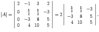
единственное решение: Hence, there are no solutions other than trivial ones. So, if there is a non-trivial solution, then r Adequacy: Let r Theorem 4.5. In order for a homogeneous system of n linear equations with n unknowns to have non-zero solutions, it is necessary and sufficient that its determinant be equal to zero, i.e. =0. If the system has nonzero solutions, then =0. For at 0 the system has only a single, zero solution. If =0, then the rank r of the main matrix of the system is less than the number of unknowns, i.e. r Example 4.6. Solve the system Putting x 3 =0, we get one particular solution: x 1 =0, x 2 =0, x 3 =0. Putting x 3 \u003d 1, we get the second particular solution: x 1 \u003d 2, x 2 \u003d 3, x 3 \u003d 1, etc. LINEAR EQUATIONS AND INEQUALITIES I § 28 Condition under which the 2nd order determinant is equal to zero In all applications of the theory of determinants, an important role is played by the conditions under which the determinant vanishes. We will consider these conditions in this section. Theorem 1. If the determinant strings proportional, then this determinant is equal to zero. Proof. Row proportionality ( a, b
) and ( c, d
) means that: or a = kc, b = kd,
or c \u003d k "a, d \u003d k" b.
(This, of course, does not rule out the possibility of both.) If a a = kc, b = kd
, then The situation is similar in the case when c \u003d k "a, d \u003d k" b
: The theorem has been proven. The converse theorem is also true. Theorem 2. If the determinant equals zero, then its rows are proportional. Proof. By condition ad - bc
= 0, ad = bc
. (1) If none of the elements of the second row ( c, d
) is not equal to zero, then it follows from (1) that a /
c
= b /
d
But this already means that the lines ( a, b
) and ( c, d
) are proportional. If both numbers with
and d
are equal to zero, then the rows of determinants will again be proportional (see problem 226 from the previous paragraph). It remains to consider only the case when one of the numbers with
and d
is zero and the other is non-zero. Let, for example, with
= 0, a d
=/= 0. Then it follows from (1) that a
= 0. But in this case, in the determinant the first column will consist of all zeros. Therefore, the rows of the determinant will be proportional (see problem 226). The proved two theorems lead to the following result. Determinant is zero if and only if its rows are proportional. Exercises
227. At what values a
the data lines of the determinants are proportional: 228. Columns of a 2nd order determinant are called proportional if at least one of them is obtained as a result of element-wise multiplication of the other by some number k
. Prove that if the rows in the 2nd order determinant are proportional, then the columns are also proportional. Is the converse true? 227
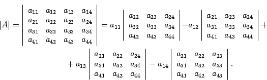
. a) ± 2; b) 0; c) for any value of o the rows of the given determinant are not proportional. The task involves familiarizing the user with the basic concepts of numerical methods, such as determinant and inverse matrix, and various ways to calculate them. In this theoretical report, in simple and accessible language, the basic concepts and definitions are first introduced, on the basis of which further research is carried out. The user may not have special knowledge in the field of numerical methods and linear algebra, but will easily be able to use the results of this work. For clarity, a program for calculating the matrix determinant by several methods, written in the C ++ programming language, is given. The program is used as a laboratory stand for creating illustrations for the report. And also a study of methods for solving systems of linear algebraic equations is being carried out. The uselessness of calculating the inverse matrix is proved, so the paper provides more optimal ways to solve equations without calculating it. It is explained why there are so many different methods for calculating determinants and inverse matrices and their shortcomings are analyzed. Errors in the calculation of the determinant are also considered and the achieved accuracy is estimated. In addition to Russian terms, their English equivalents are also used in the work to understand under what names to search for numerical procedures in libraries and what their parameters mean. Let us introduce the definition of the determinant of a square matrix of any order. This definition will recurrent, that is, to establish what the determinant of the order matrix is, you need to already know what the determinant of the order matrix is. Note also that the determinant exists only for square matrices. The determinant of a square matrix will be denoted by or det . Definition 1. determinant square matrix determinant where is the determinant of the order matrix obtained from the matrix by deleting the first row and the column with the number . For clarity, we write down how you can calculate the determinant of a matrix of the fourth order: Comment. The actual calculation of determinants for matrices above the third order based on the definition is used in exceptional cases. As a rule, the calculation is carried out according to other algorithms, which will be discussed later and which require less computational work. Comment. In Definition 1, it would be more accurate to say that the determinant is a function defined on the set of square order matrices and taking values in the set of numbers. Comment. In the literature, instead of the term "determinant", the term "determinant" is also used, which has the same meaning. From the word "determinant" the designation det appeared. Let us consider some properties of determinants, which we formulate in the form of assertions. Statement 1. When transposing a matrix, the determinant does not change, that is, . Statement 2. The determinant of the product of square matrices is equal to the product of the determinants of the factors, that is, . Statement 3. If two rows in a matrix are swapped, then its determinant will change sign. Statement 4. If a matrix has two identical rows, then its determinant is zero. In the future, we will need to add strings and multiply a string by a number. We will perform these operations on rows (columns) in the same way as operations on row matrices (column matrices), that is, element by element. The result will be a row (column), which, as a rule, does not match the rows of the original matrix. In the presence of operations of adding rows (columns) and multiplying them by a number, we can also talk about linear combinations of rows (columns), that is, sums with numerical coefficients. Statement 5. If a row of a matrix is multiplied by a number, then its determinant will be multiplied by that number. Statement 6. If the matrix contains a zero row, then its determinant is zero. Statement 7. If one of the rows of the matrix is equal to the other multiplied by a number (the rows are proportional), then the determinant of the matrix is zero. Statement 8. Let the i-th row in the matrix look like . Then , where the matrix is obtained from the matrix by replacing the i-th row with the row , and the matrix is obtained by replacing the i-th row with the row . Statement 9. If one of the rows of the matrix is added to another, multiplied by a number, then the determinant of the matrix will not change. Statement 10. If one of the rows of a matrix is a linear combination of its other rows, then the determinant of the matrix is zero. Definition 2. Algebraic addition to a matrix element is called a number equal to , where is the determinant of the matrix obtained from the matrix by deleting the i-th row and the j-th column. The algebraic complement to a matrix element is denoted by . Example. Let be Comment. Using algebraic additions, the definition of 1 determinant can be written as follows: Statement 11. Decomposition of the determinant in an arbitrary string. The matrix determinant satisfies the formula Example. Calculate Decision. Let's use the expansion in the third line, it's more profitable, because in the third line two numbers out of three are zeros. Get Statement 12. For a square matrix of order at , we have the relation Statement 13. All properties of the determinant formulated for rows (statements 1 - 11) are also valid for columns, in particular, the decomposition of the determinant in the j-th column is valid Statement 14. The determinant of a triangular matrix is equal to the product of the elements of its main diagonal. Consequence. The determinant of the identity matrix is equal to one, . Conclusion. The properties listed above make it possible to find determinants of matrices of sufficiently high orders with a relatively small amount of calculations. The calculation algorithm is the following. Algorithm for creating zeros in a column. Let it be required to calculate the order determinant . If , then swap the first line and any other line in which the first element is not zero. As a result, the determinant , will be equal to the determinant of the new matrix with the opposite sign. If the first element of each row is equal to zero, then the matrix has a zero column and, by Statements 1, 13, its determinant is equal to zero. So, we consider that already in the original matrix . Leave the first line unchanged. Let's add to the second line the first line, multiplied by the number . Then the first element of the second row will be equal to The remaining elements of the new second row will be denoted by , . The determinant of the new matrix according to Statement 9 is equal to . Multiply the first line by the number and add it to the third. The first element of the new third row will be equal to The remaining elements of the new third row will be denoted by , . The determinant of the new matrix according to Statement 9 is equal to . We will continue the process of obtaining zeros instead of the first elements of strings. Finally, we multiply the first line by a number and add it to the last line. The result is a matrix, denoted by , which has the form and . To calculate the determinant of the matrix, we use the expansion in the first column Since then The determinant of the order matrix is on the right side. We apply the same algorithm to it, and the calculation of the determinant of the matrix will be reduced to the calculation of the determinant of the order matrix. The process is repeated until we reach the second-order determinant, which is calculated by definition. If the matrix does not have any specific properties, then it is not possible to significantly reduce the amount of calculations compared to the proposed algorithm. Another good side of this algorithm is that it is easy to write a program for a computer to calculate the determinants of matrices of large orders. In standard programs for calculating determinants, this algorithm is used with minor changes associated with minimizing the effect of rounding errors and input data errors in computer calculations. Example. Compute Matrix Determinant Decision. The first line is left unchanged. To the second line we add the first, multiplied by the number: The determinant does not change. To the third line we add the first, multiplied by the number: The determinant does not change. To the fourth line we add the first, multiplied by the number: The determinant does not change. As a result, we get Using the same algorithm, we calculate the determinant of a matrix of order 3, which is on the right. We leave the first line unchanged, to the second line we add the first, multiplied by the number To the third line we add the first, multiplied by the number As a result, we get Answer. . Comment. Although fractions were used in the calculations, the result was an integer. Indeed, using the properties of determinants and the fact that the original numbers are integers, operations with fractions could be avoided. But in engineering practice, numbers are extremely rarely integers. Therefore, as a rule, the elements of the determinant will be decimal fractions and it is not advisable to use any tricks to simplify calculations. Definition 3. The matrix is called inverse matrix for a square matrix if . It follows from the definition that the inverse matrix will be a square matrix of the same order as the matrix (otherwise one of the products or would not be defined). The inverse matrix for a matrix is denoted by . Thus, if exists, then . From the definition of an inverse matrix, it follows that the matrix is the inverse of the matrix, that is, . Matrices and can be said to be inverse to each other or mutually inverse. If the determinant of a matrix is zero, then its inverse does not exist. Since for finding the inverse matrix it is important whether the determinant of the matrix is equal to zero or not, we introduce the following definitions. Definition 4. Let's call the square matrix degenerate or special matrix, if non-degenerate or nonsingular matrix, if . Statement. If an inverse matrix exists, then it is unique. Statement. If a square matrix is nondegenerate, then its inverse exists and Theorem. An inverse matrix for a square matrix exists if and only if the matrix is nonsingular, the inverse matrix is unique, and formula (1) is valid. Comment. Particular attention should be paid to the places occupied by algebraic complements in the inverse matrix formula: the first index shows the number column, and the second is the number lines, in which the calculated algebraic complement should be written. Example. Decision. Finding the determinant Since , then the matrix is nondegenerate, and the inverse for it exists. Finding algebraic additions: We compose the inverse matrix by placing the found algebraic additions so that the first index corresponds to the column, and the second to the row: The resulting matrix (2) is the answer to the problem. Comment. In the previous example, it would be more accurate to write the answer like this: However, the notation (2) is more compact and it is more convenient to carry out further calculations, if any, with it. Therefore, writing the answer in the form (2) is preferable if the elements of the matrices are integers. And vice versa, if the elements of the matrix are decimal fractions, then it is better to write the inverse matrix without a factor in front. Comment. When finding the inverse matrix, you have to perform quite a lot of calculations and an unusual rule for arranging algebraic additions in the final matrix. Therefore, there is a high chance of error. To avoid errors, you should do a check: calculate the product of the original matrix by the final one in one order or another. If the result is an identity matrix, then the inverse matrix is found correctly. Otherwise, you need to look for an error. Example. Find the inverse of a matrix Decision.
Answer: Conclusion. Finding the inverse matrix by formula (1) requires too many calculations. For matrices of the fourth order and higher, this is unacceptable. The real algorithm for finding the inverse matrix will be given later. The Gauss method can be used to find the determinant and inverse matrix. Namely, the matrix determinant is equal to det . The inverse matrix is found by solving systems of linear equations using the Gaussian elimination method: Where is the j-th column of the identity matrix , is the desired vector. The resulting solution vectors - form, obviously, the columns of the matrix, since . 1.
If the matrix is nonsingular, then and (the product of the leading elements). Since for finding the inverse matrix it is important whether the determinant of the matrix is equal to zero or not, we introduce the following definitions. Definition 14.9 Let's call the square matrix degenerate or special matrix, if non-degenerate or nonsingular matrix, if . Offer 14.21 If an inverse matrix exists, then it is unique. Proof. Let two matrices and be the inverse of the matrix . Then Hence, . Cramer's rule. Let the matrix equation AX=B Where ; is the determinant obtained from the determinant D replacement i-th column by the column of free members of the matrix B: Proof The theorem is divided into three parts: 1. The solution of system (1) exists and is unique. 2. Equalities (2) are a consequence of the matrix equation (1). 3. Equalities (2) entail matrix equation (1). Since , there also exists a unique inverse matrix . uniqueness inverse matrix proves the first part of the theorem. Let's move on to the proof one-to-one correspondence between formulas (1) and (2). Using formula (4), we obtain an expression for i-th element. For this you need to multiply i-th row of the matrix per column B. Given that i-th row of the associated matrix is composed of algebraic additions , we get the following result: The derivation of Cramer's formulas is complete. Let us now show that the expressions Let's change the order of summation on the right side of the resulting expression: where is the delta Kronecker symbol. Given that the delta symbol removes the summation over one of the indices, we get the required result: Complex numbers: The idea is to define new objects with the help of known ones. Real numbers are located on a straight line. When passing to the plane, we obtain complex numbers. Definition: A complex number is a pair of real numbers z = (a,b). The number a = Re z is called the real part, and b = Im z the imaginary part of the complex number z . Operations on complex numbers: The complex numbers z1 z2 are Z1 = z2 ⇔ Re z1 = Re z2 & Im z1 = Im z2. Addition: Z=z1+z2. ⇔Rez=Rez1+Rez2 & Imz1+ Imz2. The number (0,0) is denoted by 0. This is the neutral element. It is verified that the addition of complex numbers has properties similar to those of the addition of real numbers. (1. Z1+ z2 = z2 + z1 – commutativity; 2. Z1 + (z2 + z3) = (z1 + z2) + z3 – associativity; 3. Z1 + 0 = z1 - existence of zero (neutral element); 4. z + (−z) = 0 - the existence of the opposite element). Multiplication: z= z1 z2⇔Re z=Re z1 Re z2-Im z1 Im z2 & Im z1=Im z1 Re z2+Im z2 Re z1. A complex number z lies on the real axis if Imz = 0 . The results of operations on such numbers coincide with the results of operations on ordinary real numbers. Multiplication of complex numbers has the properties of closure, commutativity and associativity. The number (1,0) is denoted by 1. It is a neutral element by multiplication. If a∈ R, z ∈C , then Re(az) = aRe z, Im(az) = a Imz . Definition The number (0,1) is denoted by i and is called the imaginary unit. In this notation, we obtain the representation of a complex number in algebraic form: z = a + ib, a,b∈ R. i=-1.(a,b)=(a,0)+(0,b) ;(a,0)+b(0,1)=a+ib=z; (a1+ib)(a2+ib2)=a1a2+i(a1b2+1-a2b1)-b1b2; (a+ib)(1+0i)=a+ib; z(a,b), z(0+i0)=0; z!=0; a 2 + b 2 > 0 (a + ib) (a-ib / a 2 + b 2) = 1. The number is called conjugate to z if Re =Re z ; Im =-
Im z. = + ; = ; z =(a+ib)(a-ib)=a 2 +b 2 The modulus of a number z is a real number| z |= . Fair formula| z| 2 = z It follows from the definition that z ≠ 0⇔| z|≠ 0. z -1 = /|z| 2 (1) Trigonometric form of a complex number: a=rcos(t); b=r sin(t). Z=a+ib=r(cos(t)+isin(t))(2) t-argument of a complex number. Z1=z2 =>|z1|=|z2| arg(z1)-arg(z2)=2pk. Z1=r1(cos(t1)+isin(t1), Z2=r2(cos(t2)+isin(t2)), Z3=z1 z2=T1T2(cos(t1+t2)+isin(t1+t2)( one) Arg(z1z2)=arg(z1)+arg(z2) (2) Z!=0 z -1 = /|z| 2 =1/r(cos(-t)+i(sin(-t)) Z=r(cos(t)+istn(t)) R(cos(t)-isin(t)) Definition: The root of the degree n from unity is the solution of the equation z n =1 Proposal. There are n distinct nth roots of unity. They are written as z = cos(2 π k / n) + isin(2 π k / n), k = 0,..., n −1 . Theorem. In the set of complex numbers, the equation always has n solutions. Z=r(cos(t)+isin(t)); z n =r n (cos(nt)+isin(nt))=1(cos(0)+isin(0))=>z n =1 .Z-integers. K belongs to Z. k=2=E 2 =E n-1 E n ; E n =1; E n+p =E p . Thus, it is proved that the solutions of the equation are the vertices of a regular n-gon, and one of the vertices coincides with 1. nth root of z 0. Z k \u003d Z 0; Z0 =0=>Z=0; Z 0 !=0;Z=r(cos(t)-isin(t)); Z 0 \u003d r 0 (cos (t0) + isin (t0)); r0!=0; Z n \u003d r n (cos (nt) + isin (nt))
r n \u003d r 0, nt-t 0 \u003d 2pk; r=; t=(2пk+t0)/n; z= (cos((2pk+t0)/n)+isin((2pk+t0)/n)= (cos t0/n+isin t0/n)(cos(2pk/n)+isin(2pk/n) )=Z 1 E k ;z=z 1 E k ;Z 1 n =z 0, k=0, n=1 Matrices. Definition: An m × n matrix is a rectangular table containing m rows and n columns, whose elements are real or complex numbers. Matrix elements have double indices. If m = n, then it is a square matrix of order m, and elements with the same index form the main diagonal of the matrix. Matrix Operations: Definition: Two matrices A,B are called equal if their sizes are the same and A = B,1≤ i ≤ m,1≤ j ≤ n Addition. Matrices of the same size are considered. Definition:C = A + B ⇔ C = A + B, ∀i, j Offer. Matrix addition is commutative, associative, there is a neutral element and for each matrix there is an opposite element. The neutral element is the zero matrix, all elements of which are equal to 0. It is denoted by Θ. Multiplication. An m × n matrix A is denoted by Amn . Definition: C mk =A mn B nk ó C= Note that, in general, multiplication is not commutative. Closedness is valid for a square matrix of a fixed size. Let three matrices Amn , Bnk , Ckr be given. Then (AB)C = A(BC). If a product of 3 matrices exists, then it is associative. The Kronecker symbol δij . It is 1 if the indices match, and 0 otherwise. Definition. The identity matrix I n is a square matrix of order n for which the equalities n I n [ i | j] = δij Offer. Equalities I m A mn =A mn I n =A mn The addition and multiplication of matrices is connected by the laws of distributivity. A(B+C)=AB+AC; (A+B)C=AC+BC;(A(B+C)= = = + Matrix transposition. A transposed matrix is a matrix obtained from the original one by replacing rows with columns. (A+B) T = A T + B T (AB) T \u003d B T A T; (AB) T \u003d (AB) \u003d \u003d (B T A T) Multiplying a matrix by a number. The product of the number a and the matrix A mn is called the new matrix B=aA 1*A=A;a(A+B)=aA+aB;(a+b)A=aA+bA; A(BC)=(aB)C=B(aC); (ab)A=a(bA)=b(aA) linear space(L) over the field F is called the set of vectors L=(α,β..) 1.α+β=β+α(commutativity) 2.α+(β+γ)= (α+β)+γ, (ab)α=a(bα)(associativity) 3.α+θ=α, α∙1=α(existence of neutral) 4.α+(-α)=θ (existence of opposite) a(α+β)=aα+aβ, (a+b)α=aα+bα. Documentation (|(a+b)α|=|a+b||α|, |aα|=|a||α|,|bα|=|b||α|, a and b>0, |a+b|=a+b,|a|=a,|b|=b.) aα+(-a)α=θ, (a+0)α=aα An example of a linear space is a set of fixed-size matrices with operations of addition and multiplication by a number. System linear vectors called linearly dependent, if 1.a 1 ,a 2 ..a n ≠0 2. a 1 α 1 ,a 2 α 2 ..a n α n =θ If the system is not linearly dependent, then it is linearly independent. Consider 1. n=1 α 1 depend. a 1 ≠0, a 1 α 1 =θ, a 1 -1 (a 1 α 1)= a 1 -1∙ θ=θ, (a 1 -1 a 1)α 1 =1∙α 1 =α 1 ; 2. n=2 α 1 ,α 2 depend. a 1 ≠0, a 1 α 1 + a 2 α 2 =θ, α 1 = -a 1 -1 a 2 α 2 = b 2 α 2; 3.n≥2 α 1 ..α n depend. a 1 ≠0, α 1 =Σ k =2 n b k α k , 1α 1 - Σ k =2 n b k α k =θ, (1,b 2 ..b n)≠0 Offer: A system of vectors containing more than 1 vector is linearly dependent, then some vector of the system is a linear combination of the others. If a system of vectors contains a linearly dependent subsystem, then the entire system is linearly dependent. Documentation: (α 1 ..α n depend. System: α 1 ..α n ;α n +1 ..α m , a 1 α 1 +..+a n α n +0α n +1 +.. +0α m =θ, a 1 ..a n ,0..0≠0.) If the system contains a null vector, then it is linearly dependent. Linear spaces theorem: (Let 2 systems of vectors α 1 ..α m , β 1 ..β n be given. The system of vectors α is expressed in terms of β if each vector α is a linear combination β α i = Σ k =1 n a ik β k , (α ) ( (β), (β) ( (γ)→ (α) ( (γ)) Theorem: Given 2 systems of vectors, α is independent and, (α) ( (β)→m≤n Let us prove that α 1 ..α m +1 β 1 ..β m (α) ( (β)→(α) depends (Let's prove by induction. m=1: α 1 =a 11 β 1 , α 2 =a 21 β 1. a 11 =0→ α 1 =θ. a 11 α 2 – a 21 α 1 = a 11 a 21 β 1 - a 21 a 11 β 1 =θ. α 1 = a 11 β 1 +.. a 1 n -1 β n -1 .. α n = a n 1 β 1 + .. a nn -1 β n - 1 If all coefficients =0 a 11 =a 12 =..=a 1 n -1 =0→ α 1 =θ→ the whole system is linearly dependent a 1 n -1 ≠0 α 2 ′= α 2 –с 2 α 1 =b 21 β 1 +..+b 2 n -2 β n -2 , c 2 =a 2 n -1 / a 1 n -1 , α 3 ′= α 3 –с 3 α 1 .. α n ′= α n –с n α 1. By pre-induction, there exists a non-zero set of numbers d 2 ..d n: d 2 α 2 ′+d 3 α 3 ′+.. d n α n ′=θ , d 2 ( α 2 –с 2 α 1)+d 3 (α 3 –с 3 α 1)+.. d n (α n –с n α 1)=θ , (α) ( (β), m>n →(α )depend if (α) independent →m≤n) MLNP-max.line.independent.subsystem. Let a system of vectors α 1 ..α n of some subsystem be given. α i 1 ..α in is called MLIS if 1. α 1 ..α n is independent2. α i 1 ..α ir , α ij depends. Each vector of the system is a linear combination of MLLM vectors. ( α i 1 ..α ir , α ij dependent a i 1 α i 1 +.. a ir α ir +a ij α ij =θ a i 1 ..a ir , a ij ≠0 if a ij =0 → a i 1 α i 1 +.. a ir α ir =θ a i 1 ..a ir =0 contradiction a ij ≠0 α ij = a ij - 1 (-a i 1 α i 1 -.. a ir α ir) (α 1 ..α n) ( (α i 1 ..α ir) Consequence: Any 2 MLIS from one system of vectors contain the same number of vectors (α i 1 ..α ir) ( (α j 1 ..α jk) , (α j 1 ..α jk) ( (α i 1 ..α ir ) k≤r, r≤k →r=k The number of MLLM vectors is called rank original system. In the case of a linear space (a system of vectors consists of all vectors in the space), the MLLM mb is either finite or infinite. We consider the final case. The number of vectors (rank) is the dimension of the linear space. MLNP base. The space of directed segments. Two non-collinear vectors make up base in the space of vectors on the plane. α 3 = α 1 ′+ α 2 ′=a 1 α 1 + a 2 α 2 . 3 vectors linearly dependent α 3 =a 1 α 1 + a 2 α 2 . Complanarity - 3 vectors are parallel to the same plane α 4 = α 4 ′+ α 5 ′ , α 4 ′=a 1 α 1 + a 2 α 2 , α 5 ′= a 3 α 3 , α 4 = a 1 α 1 + a 2 α 2 + a 3 α 3 . Space of strings of length n. α= Offer: The space of strings of length n has dimension n. ( ξ 1 =<1…0>ξ2 =<0,1…0>.. n =<0…1>,a 1 ξ 1 + a 2 ξ 2 +.. a n ξ n =θ=<0,..0> → a 1 =a 2 =..a n =0 (linear independence) β= β= b 1 ξ 1 + b 2 ξ 2 +.. b n ξ n →the space of strings of length n has dimension and n. Matrix rank. Two systems of vectors α and β are called equivalent if each vector α( β(expressed) and β( α. Offer. The ranks of equivalent systems coincide. α i 1 , α i 2 ,…, α ir – MLLM α , β i 1 , β i 2 ,…, β ik – MLLM β , α i 1 , α i 2 ,…, α ir< β < β i 1 , β i 2 ,…, β ik → r<=k Swapping α and β places → r>=k >>> Hence, r=k. Definition. Let the matrix A= Matrix rank A is called the rank of the system of vectors α1, α2,…, αm, composed of this matrix >>rank(A)-rank From the definition, it is obvious that when the columns are rearranged, the rank does not change. Let us show that when the columns are rearranged, the rank does not change either. A'= Linear dependent: b 1 α 1 + b 2 α 2 +…+ b m α m =θ, b 1 a 11 +b 2 a 21 +…+b m a m 1=0, b 1 α' 1 + b 2 α' 2 +…+ b m α' m , b 1 a 11 +b 2 a 21 +…+b m a m 1=0 It is equal to the sum of the products of the elements of some row or column and their algebraic complements, i.e. , where i 0 is fixed. Service assignment. This service is designed to find the determinant of the matrix online with the design of the entire course of the solution in Word format. Additionally, a solution template is created in Excel. Instruction. Select the dimension of the matrix, click Next. Let's determine the minor for (2,1): to do this, we delete the second row and the first column from the matrix. Let's find the determinant using expansion by rows (by the first row):


Formulation of the problem
Basic definitions and simple properties
Determinant
 second order number is called
 ![]() .
. square matrix of order , is called the number
 . Then


 .
.
 .
. and equality
  at .
at .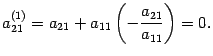 .
.


 .
.
 :
: :
:
inverse matrix
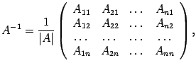 (1) where are algebraic additions to elements .
 .
.
 (2)
(2) (3)
(3) .
.![]() - exist.
- exist. .
.Calculating the determinant and inverse matrix using the Gauss method
Formulas for the determinant

Multiplying both parts of the matrix equation (1) on the left by , we obtain the solution of this equation:
![]()

The expression (*) is called the decomposition of the determinant D in terms of the elements of the row with the number i 0 .Algorithm for finding the determinant
To calculate the determinant containing functions in the matrix, standard methods are used. For example, calculate the determinant of a 3rd order matrix: 
Let's use the first line expansion.
Δ = sin(x)× + 1× = 2sin(x)cos(x)-2cos(x) = sin(2x)-2cos(x) Methods for calculating determinants
Finding the determinant through algebraic additions is a common method. Its simplified version is the calculation of the determinant by the Sarrus rule. However, with a large matrix dimension, the following methods are used:
In Excel, to calculate the determinant, the function = MOPRED (range of cells) is used. Applied use of determinants
The determinants are usually calculated for specific system, given as a square matrix. Consider some types of tasks on finding matrix determinant.
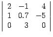
 Sometimes it is required to find an unknown parameter a for which the determinant would be equal to zero. To do this, it is necessary to draw up an equation for the determinant (for example, according to triangle rule) and, equating it to 0 , calculate the parameter a .
decomposition by columns (by the first column):
Minor for (1,1): Delete the first row and the first column from the matrix.
Let's find the determinant for this minor. ∆ 1,1 \u003d (2 (-2) -2 1) \u003d -6.
Let's find the determinant for this minor. ∆ 3,1 = (0 1-2 (-2)) = 4
The main determinant is: ∆ = (1 (-6)-3 4+1 4) = -14
Minor for (1,1): Delete the first row and the first column from the matrix.
Let's find the determinant for this minor. ∆ 1,1 \u003d (2 (-2) -2 1) \u003d -6. Minor for (1,2): Delete the 1st row and 2nd column from the matrix. Let us calculate the determinant for this minor. ∆ 1,2 \u003d (3 (-2) -1 1) \u003d -7. And to find the minor for (1,3) we delete the first row and the third column from the matrix. Let's find the determinant for this minor. ∆ 1.3 = (3 2-1 2) = 4
We find the main determinant: ∆ \u003d (1 (-6) -0 (-7) + (-2 4)) \u003d -14