Matrix method for solving a square slough. Solving systems of linear algebraic equations using an inverse matrix

Consider system of linear algebraic equations(SLOW) regarding n unknown x 1 , x 2 , ..., x n :

This system in a "folded" form can be written as follows:

S n i=1 a ij x j = b i , i=1,2, ..., n.

In accordance with the rule of matrix multiplication, the considered system linear equations can be written in matrix form ax=b, where

, ,.

Matrix A, whose columns are the coefficients for the corresponding unknowns, and the rows are the coefficients for the unknowns in the corresponding equation is called system matrix. column matrix b, whose elements are the right parts of the equations of the system, is called the matrix of the right part or simply right side of the system. column matrix x , whose elements are unknown unknowns, is called system solution.

The system of linear algebraic equations written as ax=b, is an matrix equation.

If the matrix of the system non-degenerate, then it has inverse matrix and then the solution of the system ax=b is given by the formula:

x=A -1 b.

Example Solve the system matrix method.

Decision find the inverse matrix for the coefficient matrix of the system

Calculate the determinant by expanding over the first row:

Insofar as Δ ≠ 0 , then A -1 exist.

The inverse matrix is ​​found correctly.

Let's find a solution to the system

Hence, x 1 = 1, x 2 = 2, x 3 = 3 .

Examination:

7. The Kronecker-Capelli theorem on the compatibility of a system of linear algebraic equations.

System of linear equations looks like:

a 21 x 1 + a 22 x 2 +... + a 2n x n = b 2 , (5.1)

a m1 x 1 + a m1 x 2 +... + a mn x n = b m .

Here a i j and b i (i = ; j = ) are given, and x j are unknown real numbers. Using the concept of a product of matrices, we can rewrite system (5.1) in the form:

where A = (a i j) is a matrix consisting of coefficients at unknown systems(5.1), which is called system matrix, X = (x 1 , x 2 ,..., x n) T , B = (b 1 , b 2 ,..., b m) T - column vectors composed respectively of unknown x j and free terms b i .

Ordered collection n real numbers (c 1 , c 2 ,..., c n) is called system solution(5.1) if as a result of substitution of these numbers instead of the corresponding variables x 1 , x 2 ,..., x n each equation of the system turns into an arithmetic identity; in other words, if there exists a vector C= (c 1 , c 2 ,..., c n) T such that AC  B.

System (5.1) is called joint, or solvable if it has at least one solution. The system is called incompatible, or insoluble if it has no solutions.

,

formed by assigning a column of free terms to the matrix A on the right, is called extended matrix system.

The question of the compatibility of system (5.1) is solved by the following theorem.

Kronecker-Capelli theorem . The system of linear equations is consistent if and only if the ranks of the matrices A and A coincide, i.e. r(A) = r(A) = r.

For the set M of solutions to system (5.1), there are three possibilities:

1) M =  (in this case the system is inconsistent);

2) M consists of one element, i.e. the system has a unique solution (in this case the system is called certain);

3) M consists of more than one element (then the system is called uncertain). In the third case, system (5.1) has an infinite number of solutions.

The system has a unique solution only if r(A) = n. In this case, the number of equations is not less than the number of unknowns (mn); if m>n, then m-n equations are consequences of the others. If 0

To solve an arbitrary system of linear equations, one must be able to solve systems in which the number of equations is equal to the number of unknowns, the so-called Cramer type systems:

a 11 x 1 + a 12 x 2 +... + a 1n x n = b 1 ,

a 21 x 1 + a 22 x 2 +... + a 2n x n = b 2 , (5.3)

... ... ... ... ... ...

a n1 x 1 + a n1 x 2 +... + a nn x n = b n .

Systems (5.3) are solved in one of the following ways: 1) by the Gauss method, or by the method of eliminating unknowns; 2) according to Cramer's formulas; 3) by the matrix method.

Example 2.12. Investigate the system of equations and solve it if it is compatible:

5x 1 - x 2 + 2x 3 + x 4 = 7,

2x1 + x2 + 4x3 - 2x4 = 1,

x 1 - 3x 2 - 6x 3 + 5x 4 = 0.

Decision. We write out the extended matrix of the system:

 .

Let us calculate the rank of the main matrix of the system. It is obvious that, for example, the second-order minor in the upper left corner = 7  0; the third-order minors containing it are equal to zero:

Therefore, the rank of the main matrix of the system is 2, i.e. r(A) = 2. To calculate the rank of the extended matrix A, consider the bordering minor

hence, the rank of the extended matrix is ​​r(A) = 3. Since r(A)  r(A), the system is inconsistent.

This is a concept that generalizes all possible operations performed with matrices. Mathematical matrix - a table of elements. About a table where m lines and n columns, they say that this matrix has the dimension m on the n.

General view of the matrix:

For matrix solutions you need to understand what a matrix is ​​​​and know its main parameters. The main elements of the matrix:

• Main Diagonal Consisting of Elements a 11, a 22 ..... a mn.
• Side diagonal consisting of elements а 1n ,а 2n-1 …..а m1.

The main types of matrices:

• Square - such a matrix, where the number of rows = the number of columns ( m=n).
• Zero - where all elements of the matrix = 0.
• Transposed Matrix - Matrix AT, which was obtained from the original matrix A by replacing rows with columns.
• Single - all elements of the main diagonal = 1, all others = 0.
• An inverse matrix is ​​a matrix that, when multiplied by the original matrix, results in the identity matrix.

The matrix can be symmetrical with respect to the main and secondary diagonals. That is, if a 12 = a 21, a 13 \u003d a 31, .... a 23 \u003d a 32 .... a m-1n =a mn-1, then the matrix is ​​symmetric with respect to the main diagonal. Only square matrices can be symmetric.

Methods for solving matrices.

Almost all matrix solution methods are to find its determinant n th order and most of them are quite cumbersome. To find the determinant of the 2nd and 3rd order, there are other, more rational ways.

Finding determinants of the 2nd order.

To calculate the matrix determinant BUT 2nd order, it is necessary to subtract the product of the elements of the secondary diagonal from the product of the elements of the main diagonal:

Methods for finding determinants of the 3rd order.

Below are the rules for finding the 3rd order determinant.

Simplified the triangle rule as one of matrix solution methods, can be represented as follows:

In other words, the product of elements in the first determinant that are connected by lines is taken with a "+" sign; also, for the 2nd determinant - the corresponding products are taken with the "-" sign, that is, according to the following scheme:

At solving matrices by the Sarrus rule, to the right of the determinant, the first 2 columns are added and the products of the corresponding elements on the main diagonal and on the diagonals that are parallel to it are taken with a "+" sign; and the products of the corresponding elements of the secondary diagonal and the diagonals that are parallel to it, with the sign "-":

Row or column expansion of determinant when solving matrices.

The determinant is equal to the sum of the products of the elements of the row of the determinant and their algebraic complements. Usually choose the row/column in which/th there are zeros. The row or column on which the decomposition is carried out will be indicated by an arrow.

Reducing the determinant to a triangular form when solving matrices.

At solving matrices By reducing the determinant to a triangular form, they work like this: using the simplest transformations on rows or columns, the determinant becomes triangular and then its value, in accordance with the properties of the determinant, will be equal to the product of the elements that stand on the main diagonal.

Laplace's theorem for solving matrices.

When solving matrices using Laplace's theorem, it is necessary to know the theorem itself directly. Laplace's theorem: Let Δ is a determinant n-th order. We select any k rows (or columns), provided k≤ n - 1. In this case, the sum of the products of all minors k th order contained in the selected k rows (columns), their algebraic additions will be equal to the determinant.

Inverse matrix solution.

Sequence of actions for inverse matrix solutions:

1. Find out if the given matrix is ​​square. In the case of a negative answer, it becomes clear that there cannot be an inverse matrix for it.
2. We calculate algebraic additions.
3. We compose the allied (mutual, attached) matrix C.
4. We compose an inverse matrix from algebraic additions: all elements of the adjoint matrix C divide by the determinant of the initial matrix. The resulting matrix will be the desired inverse matrix with respect to the given one.
5. We check the work done: we multiply the matrix of the initial and the resulting matrices, the result should be the identity matrix.

Solution of matrix systems.

For solutions of matrix systems most commonly used is the Gauss method.

The Gauss method is a standard way to solve systems of linear algebraic equations (SLAE) and it consists in the fact that variables are sequentially eliminated, i.e., with the help of elementary changes, the system of equations is brought to an equivalent system of a triangular form and from it, sequentially, starting from the last (by number), find each element of the system.

Gauss method is the most versatile and best tool for finding matrix solutions. If the system has an infinite number of solutions or the system is incompatible, then it cannot be solved using Cramer's rule and the matrix method.

The Gauss method also implies direct (reduction of the extended matrix to a stepped form, i.e. getting zeros under the main diagonal) and reverse (getting zeros over the main diagonal of the extended matrix) moves. The forward move is the Gauss method, the reverse is the Gauss-Jordan method. The Gauss-Jordan method differs from the Gauss method only in the sequence of elimination of variables.

Matrix method SLAU solutions used to solve systems of equations in which the number of equations corresponds to the number of unknowns. The method is best used for solving low-order systems. The matrix method for solving systems of linear equations is based on the application of the properties of matrix multiplication.

This way, in other words inverse matrix method, called so, since the solution is reduced to the usual matrix equation, for the solution of which you need to find the inverse matrix.

Matrix solution method A SLAE with a determinant greater than or less than zero is as follows:

Suppose there is a SLE (system of linear equations) with n unknown (over an arbitrary field):

So, it is easy to translate it into a matrix form:

AX=B, where A is the main matrix of the system, B and X- columns of free members and solutions of the system, respectively:

Multiply this matrix equation on the left by A -1- inverse matrix to matrix A: A −1 (AX)=A −1 B.

Because A −1 A=E, means, X=A −1 B. The right side of the equation gives a column of solutions to the initial system. The condition for the applicability of the matrix method is the nondegeneracy of the matrix A. A necessary and sufficient condition for this is that the determinant of the matrix A:

detA≠0.

For homogeneous system of linear equations, i.e. if vector B=0, the opposite rule holds: the system AX=0 is a non-trivial (i.e., not equal to zero) solution only when detA=0. This connection between the solutions of homogeneous and inhomogeneous systems of linear equations is called alternative to Fredholm.

Thus, the solution of the SLAE by the matrix method is made according to the formula . Or, the SLAE solution is found using inverse matrix A -1.

It is known that a square matrix BUT order n on the n there is an inverse matrix A -1 only if its determinant is nonzero. Thus the system n linear algebraic equations with n unknowns are solved by the matrix method only if the determinant of the main matrix of the system is not equal to zero.

Despite the fact that there are restrictions on the possibility of using this method and there are computational difficulties for large values ​​of the coefficients and high-order systems, the method can be easily implemented on a computer.

An example of solving an inhomogeneous SLAE.

First, let's check whether the determinant of the matrix of coefficients for unknown SLAEs is not equal to zero.

Now we find alliance matrix, transpose it and substitute it into the formula for determining the inverse matrix.

We substitute the variables in the formula:

Now we find the unknowns by multiplying the inverse matrix and the column of free terms.

So, x=2; y=1; z=4.

When moving from the usual form of SLAE to the matrix form, be careful with the order of unknown variables in the system equations. for example:

DO NOT write as:

It is necessary, first, to order the unknown variables in each equation of the system and only after that proceed to the matrix notation:

In addition, you need to be careful with the designation of unknown variables, instead of x 1 , x 2 , …, x n there may be other letters. For example:

in matrix form, we write:

Using the matrix method, it is better to solve systems of linear equations in which the number of equations coincides with the number of unknown variables and the determinant of the main matrix of the system is not equal to zero. When there are more than 3 equations in the system, it will take more computational effort to find the inverse matrix, therefore, in this case, it is advisable to use the Gauss method to solve.

This online calculator solves a system of linear equations using the matrix method. A very detailed solution is given. To solve a system of linear equations, select the number of variables. Choose a method for calculating the inverse matrix. Then enter the data in the cells and click on the "Calculate" button.

×

A warning

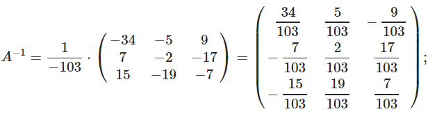
Clear all cells?

Close Clear

Data entry instruction. Numbers are entered as whole numbers (examples: 487, 5, -7623, etc.), decimal numbers (eg. 67., 102.54, etc.) or fractions. The fraction must be typed as a/b, where a and b are whole or decimal numbers. Examples 45/5, 6.6/76.4, -7/6.7, etc.

Matrix method for solving systems of linear equations

Consider the following system of linear equations:

Taking into account the definition of the inverse matrix, we have A −1 A=E, where E is the identity matrix. Therefore, (4) can be written as follows:

Thus, to solve the system of linear equations (1) (or (2)), it suffices to multiply the inverse to A matrix per constraint vector b.

Examples of solving a system of linear equations by the matrix method

Example 1. Solve the following system of linear equations using the matrix method:

Let's find the inverse to the matrix A by the Jordan-Gauss method. On the right side of the matrix A write the identity matrix:

Let's exclude the elements of the 1st column of the matrix below the main diagonal. To do this, add rows 2,3 with row 1, multiplied by -1/3, -1/3, respectively:

Let's exclude the elements of the 2nd column of the matrix below the main diagonal. To do this, add line 3 with line 2 multiplied by -24/51:

Let's exclude the elements of the 2nd column of the matrix above the main diagonal. To do this, add row 1 with row 2, multiplied by -3/17:

Separate the right side of the matrix. The resulting matrix is ​​the inverse of A :

Matrix form of writing a system of linear equations: ax=b, where

Compute all algebraic complements of the matrix A:

,

,

,

,

,

,

,

,

.

The inverse matrix is ​​calculated from the following expression.

Let there be a square matrix of the nth order

Matrix A -1 is called inverse matrix with respect to the matrix A, if A * A -1 = E, where E is the identity matrix of the nth order.

Identity matrix- such a square matrix, in which all elements along the main diagonal, passing from the upper left corner to the lower right corner, are ones, and the rest are zeros, for example:

inverse matrix may exist only for square matrices those. for those matrices that have the same number of rows and columns.

Inverse Matrix Existence Condition Theorem

For a matrix to have an inverse matrix, it is necessary and sufficient that it be nondegenerate.

The matrix A = (A1, A2,...A n) is called non-degenerate if the column vectors are linearly independent. The number of linearly independent column vectors of a matrix is ​​called the rank of the matrix. Therefore, we can say that in order for an inverse matrix to exist, it is necessary and sufficient that the rank of the matrix is ​​equal to its dimension, i.e. r = n.

Algorithm for finding the inverse matrix

1. Write the matrix A in the table for solving systems of equations by the Gauss method and on the right (in place of the right parts of the equations) assign matrix E to it.
2. Using Jordan transformations, bring matrix A to a matrix consisting of single columns; in this case, it is necessary to simultaneously transform the matrix E.
3. If necessary, rearrange the rows (equations) of the last table so that the identity matrix E is obtained under the matrix A of the original table.
4. Write the inverse matrix A -1, which is in the last table under the matrix E of the original table.

For matrix A, find the inverse matrix A -1

Solution: We write down the matrix A and on the right we assign the identity matrix E. Using Jordan transformations, we reduce the matrix A to the identity matrix E. The calculations are shown in Table 31.1.

Let's check the correctness of the calculations by multiplying the original matrix A and the inverse matrix A -1.

As a result of matrix multiplication, the identity matrix is ​​obtained. Therefore, the calculations are correct.

Answer:

Solution of matrix equations

Matrix equations can look like:

AX = B, XA = B, AXB = C,

where A, B, C are given matrices, X is the desired matrix.

Matrix equations are solved by multiplying the equation by inverse matrices.

For example, to find the matrix from an equation, you need to multiply this equation by on the left.

Therefore, to find a solution to the equation, you need to find the inverse matrix and multiply it by the matrix on the right side of the equation.

Other equations are solved similarly.

Solve the equation AX = B if

Decision: Since the inverse of the matrix equals (see example 1)

Matrix method in economic analysis

Along with others, they also find application matrix methods. These methods are based on linear and vector-matrix algebra. Such methods are used for the purposes of analyzing complex and multidimensional economic phenomena. Most often, these methods are used when it is necessary to compare the functioning of organizations and their structural divisions.

In the process of applying matrix methods of analysis, several stages can be distinguished.

At the first stage the formation of a system of economic indicators is carried out and on its basis a matrix of initial data is compiled, which is a table in which system numbers are shown in its individual lines (i = 1,2,....,n), and along the vertical graphs - numbers of indicators (j = 1,2,....,m).

At the second stage for each vertical column, the largest of the available values ​​of the indicators is revealed, which is taken as a unit.

After that, all the amounts reflected in this column are divided by the largest value and a matrix of standardized coefficients is formed.

At the third stage all components of the matrix are squared. If they have different significance, then each indicator of the matrix is ​​assigned a certain weighting coefficient k. The value of the latter is determined by an expert.

On the last fourth stage found values ​​of ratings Rj grouped in order of increasing or decreasing.

The above matrix methods should be used, for example, in a comparative analysis of various investment projects, as well as in assessing other economic performance indicators of organizations.