Excel standard deviation. Calculation of variance, root mean square (standard) deviation, coefficient of variation in Excel

Let's calculate inMSEXCELvariance and standard deviation of the sample. We also calculate the variance random variable if its distribution is known.

First consider dispersion, then standard deviation.

Sample variance

Sample variance (sample variance,samplevariance) characterizes the spread of values ​​in the array relative to .

All 3 formulas are mathematically equivalent.

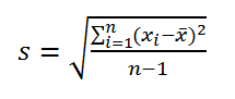
It can be seen from the first formula that sample variance is the sum of the squared deviations of each value in the array from average divided by the sample size minus 1.

dispersion samples the DISP() function is used, eng. the name of the VAR, i.e. VARIance. Since MS EXCEL 2010, it is recommended to use its analogue DISP.V() , eng. the name VARS, i.e. Sample Variance. In addition, starting from the version of MS EXCEL 2010, there is a DISP.G () function, eng. VARP name, i.e. Population VARIance which calculates dispersion for population . The whole difference comes down to the denominator: instead of n-1 like DISP.V() , DISP.G() has just n in the denominator. Prior to MS EXCEL 2010, the VARP() function was used to calculate the population variance.

Sample variance
=SQUARE(Sample)/(COUNT(Sample)-1)
=(SUMSQ(Sample)-COUNT(Sample)*AVERAGE(Sample)^2)/ (COUNT(Sample)-1)- the usual formula
=SUM((Sample -AVERAGE(Sample))^2)/ (COUNT(Sample)-1) –

Sample variance is equal to 0 only if all values ​​are equal to each other and, accordingly, are equal mean value. Usually, the larger the value dispersion, the greater the spread of values ​​in the array.

Sample variance is a point estimate dispersion distribution of the random variable from which the sample. About construction confidence intervals when evaluating dispersion can be read in the article.

Variance of a random variable

To calculate dispersion random variable, you need to know it.

For dispersion random variable X often use the notation Var(X). Dispersion is equal to the square of the deviation from the mean E(X): Var(X)=E[(X-E(X)) 2 ]

dispersion calculated by the formula:

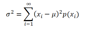
where x i is the value that the random variable can take, and μ is the average value (), p(x) is the probability that the random variable will take the value x.

If the random variable has , then dispersion calculated by the formula:

Dimension dispersion corresponds to the square of the unit of measurement of the original values. For example, if the values ​​in the sample are measurements of the weight of the part (in kg), then the dimension of the variance would be kg 2 . This can be difficult to interpret, therefore, to characterize the spread of values, a value equal to the square root of dispersion – standard deviation.

Some properties dispersion:

Var(X+a)=Var(X), where X is a random variable and a is a constant.

Var(aХ)=a 2 Var(X)

Var(X)=E[(X-E(X)) 2 ]=E=E(X 2)-E(2*X*E(X))+(E(X)) 2=E(X 2)- 2*E(X)*E(X)+(E(X)) 2 =E(X 2)-(E(X)) 2

This dispersion property is used in article about linear regression.

Var(X+Y)=Var(X) + Var(Y) + 2*Cov(X;Y), where X and Y are random variables, Cov(X;Y) is the covariance of these random variables.

If random variables are independent, then their covariance is 0, and hence Var(X+Y)=Var(X)+Var(Y). This property of the variance is used in the output.

Let us show that for independent quantities Var(X-Y)=Var(X+Y). Indeed, Var(X-Y)= Var(X-Y)= Var(X+(-Y))= Var(X)+Var(-Y)= Var(X)+Var(-Y)= Var( X)+(-1) 2 Var(Y)= Var(X)+Var(Y)= Var(X+Y). This property of the variance is used to plot .

Sample standard deviation

Sample standard deviation is a measure of how widely scattered the values ​​in the sample are relative to their .

A-priory, standard deviation equals the square root of dispersion:

Standard deviation does not take into account the magnitude of the values ​​in sampling, but only the degree of scattering of values ​​around them middle. Let's take an example to illustrate this.

Let's calculate the standard deviation for 2 samples: (1; 5; 9) and (1001; 1005; 1009). In both cases, s=4. It is obvious that the ratio of the magnitude standard deviation to the values ​​of the array, the samples differ significantly. For such cases, use The coefficient of variation(Coefficient of Variation, CV) - ratio standard deviation to the average arithmetic, expressed as a percentage.

In MS EXCEL 2007 and earlier versions for calculation Sample standard deviation the function =STDEV() is used, eng. the name STDEV, i.e. standard deviation. Since MS EXCEL 2010, it is recommended to use its analogue = STDEV.B () , eng. name STDEV.S, i.e. Sample STandard DEViation.

In addition, starting from the version of MS EXCEL 2010, there is a function STDEV.G () , eng. name STDEV.P, i.e. Population STandard DEViation which calculates standard deviation for population. The whole difference comes down to the denominator: instead of n-1 like STDEV.V() , STDEV.G() has just n in the denominator.

Standard deviation can also be calculated directly from the formulas below (see example file)
=SQRT(SQUADROTIV(Sample)/(COUNT(Sample)-1))
=SQRT((SUMSQ(Sample)-COUNT(Sample)*AVERAGE(Sample)^2)/(COUNT(Sample)-1))

Other dispersion measures

The SQUADRIVE() function calculates with umm of squared deviations of values ​​from their middle. This function will return the same result as the formula =VAR.G( Sample)*CHECK( Sample) , where Sample- a reference to a range containing an array of sample values ​​(). Calculations in the QUADROTIV() function are made according to the formula:

The SROOT() function is also a measure of the scatter of a set of data. The SIROTL() function calculates the average of the absolute values ​​of the deviations of values ​​from middle. This function will return the same result as the formula =SUMPRODUCT(ABS(Sample-AVERAGE(Sample)))/COUNT(Sample), where Sample- a reference to a range containing an array of sample values.

Calculations in the function SROOTKL () are made according to the formula:

Statistics uses a huge number of indicators, and one of them is the calculation of variance in Excel. If you do it yourself manually, it will take a lot of time, you can make a lot of mistakes. Today we will look at how to decompose mathematical formulas on the simple functions. Let's look at some of the simplest, fastest and most convenient calculation methods that will allow you to do everything in a matter of minutes.

Computing the variance

The variance of a random variable is called expected value the square of the deviation of a random variable from its mathematical expectation.

We calculate by the general population

To calculate mat. expectation in the program, the function VARI.G will be used, and its syntax is as follows "= VARI.G (Number1; Number2; ...)".

It is possible to apply a maximum of 255 arguments, no more. Arguments can be prime numbers or links to the cells in which they are specified. Let's look at how to calculate the variance in Microsoft Excel:

1. The first step is to select the cell where the result of the calculations will be displayed, and then click on the "Insert function" button.

2. The feature management shell will open. There you need to look for the function "DISP.G", which can be in the category "Statistical" or "Full alphabetical list". When it is found, select it and click OK.

3. The function arguments window will open. In it, you need to select the line "Number 1" and on the sheet select a range of cells with a number series.

4. After that, in the cell where the function was entered, the results of the calculations will be displayed.

This is how you can easily find the variance in Excel.

Making a sample calculation

In this case, the sample variance in Excel is calculated with the denominator indicating not the total number of numbers, but one less. This is done for a smaller error using the special function VAR.V, the syntax of which is =VAR.V(Number1;Number2;…). Action algorithm:

• As in the previous method, you need to select a cell for the result.
• In the function wizard, you should find "VAR.V" in the category "Full alphabetical list" or "Statistical".

• Next, a window will appear, and you should proceed in the same way as in the previous method.

Video: Calculate variance in Excel

Conclusion

The variance in Excel is calculated very simply, much faster and more convenient than doing it manually, because the mathematical expectation function is quite complicated and it can take a lot of time and effort to calculate it.

Management intervention is needed to identify the causes of deviations.

To build a control chart, I use the original data, the mean (μ) and the standard deviation (σ). In Excel: μ = AVERAGE($F$3:$F$15), σ = STDEV($F$3:$F$15)

The control chart itself includes: raw data, mean (μ), lower control limit (μ - 2σ) and upper control limit (μ + 2σ):

Download note in format , examples in format

Looking at this map, I noticed that the original data shows a very distinct linear trend towards a decrease in the overhead share:

To add a trend line, select the data row on the chart (in our example, green dots), right-click and select the "Add trend line" option. In the Format Trendline window that opens, experiment with the options. I settled on a linear trend.

If the initial data are not scattered in accordance with around the average value, then it is not quite correct to describe them by the parameters μ and σ. Instead of an average value, a straight line is better for describing linear trend and control boundaries equidistant from this trend line.

Excel allows you to build a trend line using the FORECAST function. We will need an additional row A3: A15 in order to known X values were continuous row(numbers of quarters such continuous series do not form). Instead of the average value in column H, we introduce the FORECAST function:

The standard deviation σ (STDEV function in Excel) is calculated by the formula:

Unfortunately, I did not find Excel Functions for such a definition of the standard deviation (with respect to the trend). The problem can be solved using an array formula. Who is not familiar with array formulas, I suggest reading first.

An array formula can return a single value or an array. In our case, the array formula will return a single value:

Let's take a closer look at how the array formula works in cell G3

SUM(($F$3:$F$15-$H$3:$H$15)^2) defines the sum of squared differences; in fact, the formula calculates the following sum = (F3 - H3) 2 + (F4 - H4) 2 + ... + (F15 - H15) 2

COUNT($F$3:$F$15) – number of values ​​in range F3:F15

SQRT(SUM(($F$3:$F$15-$H$3:$H$15)^2)/(COUNT($F$3:$F$15)-1)) = σ

The value of 6.2% is the point of the lower control limit = 8.3% - 2 σ

Curly quotation marks on either side of a formula indicate that it is an array formula. To create an array formula, after entering the formula in cell G3:

H4 - 2*ROOT(SUM(($F$3:$F$15-$H$3:$H$15)^2)/(COUNT($F$3:$F$15)-1))

you need to press not Enter, but Ctrl + Shift + Enter. Don't try to type curly braces on the keyboard - the array formula won't work. If you want to edit an array formula, do it in the same way as with a regular formula, but again, after editing, press Ctrl + Shift + Enter instead of Enter.

An array formula that returns a single value can be "dragged" just like a regular formula.

As a result, we got a control chart built for data with a downward trend.

P.S. After the note was written, I was able to refine the formulas used to calculate the standard deviation for data with a trend. You can get acquainted with them in the Excel file.

We have to deal with the calculation of such values ​​as variance, average standard deviation and, of course, the coefficient of variation. It is the calculation of the latter that should be given special attention. It is very important that every beginner who is just starting to work with a spreadsheet editor can quickly calculate the relative scatter of values.

What is the coefficient of variation and why is it needed?

So, it seems to me that it would be useful to conduct a short theoretical digression and understand the nature of the coefficient of variation. This indicator is necessary to reflect the range of data relative to the average value. In other words, it shows the ratio of the standard deviation to the mean. It is customary to measure the coefficient of variation in percentage terms and use it to display the homogeneity of the time series.

The coefficient of variation will become an indispensable assistant in the event that you need to make a forecast based on data from a given sample. This indicator will highlight the main ranges of values ​​that will be most useful for subsequent forecasting, as well as clear the sample from insignificant factors. So, if you see that the value of the coefficient is 0%, then declare with confidence that the series is homogeneous, which means that all values ​​in it are equal to one another. If the coefficient of variation takes on a value exceeding 33%, then this indicates that you are dealing with a heterogeneous series in which individual values ​​differ significantly from the sample average.

How to find the standard deviation?

Since we need to use the standard deviation to calculate the variation indicator in Excel, it would be quite appropriate to figure out how we calculate this parameter.

From the school algebra course, we know that the standard deviation is extracted from the variance Square root, that is, this indicator determines the degree of deviation of a particular indicator of the total sample from its average value. With its help, we can measure the absolute measure of fluctuation of the trait under study and interpret it clearly.

Calculate the coefficient in Excel

Unfortunately, Excel does not have a standard formula that would allow you to calculate the variation indicator automatically. But this does not mean that you have to do the calculations in your head. The absence of a template in the "Formula Bar" in no way detracts from Excel's abilities, so you can easily force the program to perform the calculation you need by manually typing the appropriate command.

In order to calculate the variation indicator in Excel, you need to remember the school math course and divide the standard deviation by the sample mean. That is, in fact, the formula looks like this - STDEV(specified data range) / AVERAGE(specified data range). You need to enter this formula in the Excel cell in which you want to get the calculation you need.

Keep in mind that since the coefficient is expressed as a percentage, the cell with the formula will need to be formatted accordingly. You can do this in the following way:

1. Open the Home tab.
2. Find the category in it " Format Cells"And select the required option.

Alternatively, you can set the percentage format to the cell by clicking on the right mouse button on the activated table cell. In the context menu that appears, similarly to the above algorithm, you need to select the “Cell Format” category and set the required value.

Select "Percentage" and optionally enter the number of decimal places

Perhaps the above algorithm will seem complicated to someone. In fact, calculating the coefficient is as simple as adding two natural numbers. Once you complete this task in Excel, you will never return to tedious multi-syllabic solutions in a notebook.

Still can't do qualitative comparison degree of data scatter? Lost in sample size? Then right now get down to business and master in practice all the theoretical material that was presented above! Let be statistical analysis and the development of a forecast no longer causes you fear and negativity. Save your energy and time with

Instruction

Let there be several numbers characterizing - or homogeneous quantities. For example, the results of measurements, weighings, statistical observations, etc. All quantities presented must be measured by the same measurement. To find the standard deviation, do the following.

Determine the arithmetic mean of all numbers: add all the numbers and divide the sum by total numbers.

Determine the dispersion (scatter) of numbers: add up the squares of the deviations found earlier and divide the resulting sum by the number of numbers.

There are seven patients in the ward with a temperature of 34, 35, 36, 37, 38, 39 and 40 degrees Celsius.

It is required to determine the average deviation from the average.
Decision:
"in the ward": (34+35+36+37+38+39+40)/7=37 ºС;

Temperature deviations from the average (in this case, the normal value): 34-37, 35-37, 36-37, 37-37, 38-37, 39-37, 40-37, it turns out: -3, -2, -1 , 0, 1, 2, 3 (ºС);

Divide the sum of numbers obtained earlier by their number. For the accuracy of the calculation, it is better to use a calculator. The result of the division is the arithmetic mean of the summands.

Pay close attention to all stages of the calculation, as an error in at least one of the calculations will lead to an incorrect final indicator. Check the received calculations at each stage. The average arithmetic number has the same meter as the summands of the numbers, that is, if you determine the average attendance, then all indicators will be “person”.

This method calculation is used only in mathematical and statistical calculations. So, for example, the arithmetic mean in computer science has a different calculation algorithm. The arithmetic mean is a very conditional indicator. It shows the probability of an event, provided that it has only one factor or indicator. For the most in-depth analysis, many factors must be taken into account. For this, the calculation of more general quantities is used.

The arithmetic mean is one of the measures of central tendency, widely used in mathematics and statistical calculations. Finding the arithmetic average for several values ​​​​is very simple, but each task has its own nuances, which are simply necessary to know in order to perform correct calculations.

Quantitative results of such experiments.

How to find the arithmetic mean

Features of working with negative numbers

1. Finding the common arithmetic mean by the standard method;
2. Finding the arithmetic mean of negative numbers.
3. Calculation of the arithmetic mean of positive numbers.

The responses of each of the actions are written separated by commas.

Natural and decimal fractions

When working with natural fractions, they should be reduced to a common denominator, which is multiplied by the number of numbers in the array. The numerator of the answer will be the sum of the given numerators of the original fractional elements.