What does the confidence interval show. Confidence interval

Let's build a confidence interval in MS EXCEL for estimating the mean value of the distribution in the case of a known value of the variance.

Of course the choice level of trust completely depends on the task at hand. Thus, the degree of confidence of the air passenger in the reliability of the aircraft, of course, should be higher than the degree of confidence of the buyer in the reliability of the light bulb.

Task Formulation

Let's assume that from population having taken sample size n. It is assumed that standard deviation this distribution is known. Necessary on the basis of this samples evaluate the unknown distribution mean(μ, ) and construct the corresponding bilateral confidence interval.

Point Estimation

As is known from statistics(let's call it X cf) is an unbiased estimate of the mean this population and has the distribution N(μ;σ 2 /n).

Note: What if you need to build confidence interval in the case of distribution, which is not normal? In this case, comes to the rescue, which says that with enough big size samples n from distribution non- normal, sampling distribution of statistics Х av will approximately correspond normal distribution with parameters N(μ;σ 2 /n).

So, point estimate middle distribution values we have is sample mean, i.e. X cf. Now let's get busy confidence interval.

Building a confidence interval

Usually, knowing the distribution and its parameters, we can calculate the probability that a random variable will take a value from the interval we specified. Now let's do the opposite: find the interval in which the random variable falls with a given probability. For example, from properties normal distribution it is known that with a probability of 95%, a random variable distributed over normal law, will fall within the interval approximately +/- 2 from mean value(see article about). This interval will serve as our prototype for confidence interval .

Now let's see if we know the distribution , to calculate this interval? To answer the question, we must specify the form of distribution and its parameters.

We know the form of distribution is normal distribution(remember that we are talking about sampling distribution statistics X cf).

The parameter μ is unknown to us (it just needs to be estimated using confidence interval), but we have its estimate X cf, calculated based on sample, which can be used.

The second parameter is sample mean standard deviation will be known, it is equal to σ/√n.

Because we do not know μ, then we will build the interval +/- 2 standard deviations not from mean value, but from its known estimate X cf. Those. when calculating confidence interval we will NOT assume that X cf will fall within the interval +/- 2 standard deviations from μ with a probability of 95%, and we will assume that the interval is +/- 2 standard deviations from X cf with a probability of 95% will cover μ - the average of the general population, from which sample. These two statements are equivalent, but the second statement allows us to construct confidence interval.

In addition, we refine the interval: a random variable distributed over normal law, with a 95% probability falls within the interval +/- 1.960 standard deviations, not +/- 2 standard deviations. This can be calculated using the formula \u003d NORM.ST.OBR ((1 + 0.95) / 2), cm. sample file Sheet Spacing.

Now we can formulate a probabilistic statement that will serve us to form confidence interval:
"The probability that population mean located from sample average within 1.960" standard deviations of the sample mean", is equal to 95%.

The probability value mentioned in the statement has a special name , which is associated with significance level α (alpha) by a simple expression trust level =1 -α . In our case significance level α =1-0,95=0,05 .

Now, based on this probabilistic statement, we write an expression for calculating confidence interval:

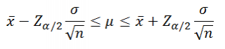
where Zα/2 – standard normal distribution(such a value random variable z, what P(z>=Zα/2 )=α/2).

Note: Upper α/2-quantile defines the width confidence interval in standard deviations sample mean. Upper α/2-quantile standard normal distribution is always greater than 0, which is very convenient.

In our case, at α=0.05, upper α/2-quantile equals 1.960. For other significance levels α (10%; 1%) upper α/2-quantile Zα/2 can be calculated using the formula \u003d NORM.ST.OBR (1-α / 2) or, if known trust level, =NORM.ST.OBR((1+confidence level)/2).

Usually when building confidence intervals for estimating the mean use only upper α/2-quantile and do not use lower α/2-quantile. This is possible because standard normal distribution symmetrical about the x-axis ( density of its distribution symmetrical about average, i.e. 0). Therefore, there is no need to calculate lower α/2-quantile(it is simply called α /2-quantile), because it is equal upper α/2-quantile with a minus sign.

Recall that, regardless of the shape of the distribution of x, the corresponding random variable X cf distributed approximately fine N(μ;σ 2 /n) (see article about). Therefore, in general, the above expression for confidence interval is only approximate. If x is distributed over normal law N(μ;σ 2 /n), then the expression for confidence interval is accurate.

Calculation of confidence interval in MS EXCEL

Let's solve the problem.
The response time of an electronic component to an input signal is an important characteristic of a device. An engineer wants to plot a confidence interval for the average response time at a confidence level of 95%. From previous experience, the engineer knows that the standard deviation of the response time is 8 ms. It is known that the engineer made 25 measurements to estimate the response time, the average value was 78 ms.

Decision: An engineer wants to know the response time of an electronic device, but he understands that the response time is not fixed, but a random variable that has its own distribution. So the best he can hope for is to determine the parameters and shape of this distribution.

Unfortunately, from the condition of the problem, we do not know the form of the distribution of the response time (it does not have to be normal). , this distribution is also unknown. Only he is known standard deviationσ=8. Therefore, while we cannot calculate the probabilities and construct confidence interval.

However, although we do not know the distribution time separate response, we know that according to CPT, sampling distribution average response time is approximately normal(we will assume that the conditions CPT are performed, because the size samples large enough (n=25)) .

Furthermore, the average this distribution is equal to mean value unit response distributions, i.e. μ. BUT standard deviation of this distribution (σ/√n) can be calculated using the formula =8/ROOT(25) .

It is also known that the engineer received point estimate parameter μ equal to 78 ms (X cf). Therefore, now we can calculate the probabilities, because we know the distribution form ( normal) and its parameters (Х ср and σ/√n).

Engineer wants to know expected valueμ of the response time distribution. As stated above, this μ is equal to expectation of the sample distribution of the average response time. If we use normal distribution N(X cf; σ/√n), then the desired μ will be in the range +/-2*σ/√n with a probability of approximately 95%.

Significance level equals 1-0.95=0.05.

Finally, find the left and right border confidence interval.
Left border: \u003d 78-NORM.ST.INR (1-0.05 / 2) * 8 / ROOT (25) = 74,864
Right border: \u003d 78 + NORM. ST. OBR (1-0.05 / 2) * 8 / ROOT (25) \u003d 81.136

Left border: =NORM.INV(0.05/2, 78, 8/SQRT(25))
Right border: =NORM.INV(1-0.05/2, 78, 8/SQRT(25))

Answer: confidence interval at 95% confidence level and σ=8msec equals 78+/-3.136ms

AT example file on sheet Sigma known created a form for calculation and construction bilateral confidence interval for arbitrary samples with a given σ and significance level.

CONFIDENCE.NORM() function

If the values samples are in the range B20:B79 , a significance level equal to 0.05; then MS EXCEL formula:
=AVERAGE(B20:B79)-CONFIDENCE(0.05,σ, COUNT(B20:B79))
will return the left border confidence interval.

The same boundary can be calculated using the formula:
=AVERAGE(B20:B79)-NORM.ST.INV(1-0.05/2)*σ/SQRT(COUNT(B20:B79))

Note: The TRUST.NORM() function appeared in MS EXCEL 2010. Earlier versions of MS EXCEL used the TRUST() function.

Let us have a large number of items with a normal distribution of some characteristics (for example, a full warehouse of the same type of vegetables, the size and weight of which varies). You want to know the average characteristics of the entire batch of goods, but you have neither the time nor the inclination to measure and weigh each vegetable. You understand that this is not necessary. But how many pieces would you need to take for random inspection?

Before giving some formulas useful for this situation, we recall some notation.

First, if we did measure the entire warehouse of vegetables (this set of elements is called the general population), then we would know with all the accuracy available to us the average value of the weight of the entire batch. Let's call this average X cf .g en . - general average. We already know what is completely determined if its mean value and deviation s are known . True, so far we are neither X avg. nor s we do not know the general population. We can only take some sample, measure the values ​​we need and calculate for this sample both the mean value X sr. in sample and the standard deviation S sb.

It is known that if our custom check contains a large number of elements (usually n is greater than 30), and they are taken really random, then s the general population will almost not differ from S ..

In addition, for the case of a normal distribution, we can use the following formulas:

With a probability of 95%

With a probability of 99%

AT general view with probability Р (t)

The relationship between the value of t and the value of the probability P (t), with which we want to know the confidence interval, can be taken from the following table:

Thus, we have determined in what range the average value for the general population is (with a given probability).

Unless we have a large enough sample, we cannot claim that the population has s = S sel. In addition, in this case, the closeness of the sample to the normal distribution is problematic. In this case, also use S sb instead s in the formula:

but the value of t for a fixed probability P(t) will depend on the number of elements in the sample n. The larger n, the closer the resulting confidence interval will be to the value given by formula (1). The values ​​of t in this case are taken from another table ( Student's t-test), which we present below:

Student's t-test values ​​for probability 0.95 and 0.99

Example 3 30 people were randomly selected from the employees of the company. According to the sample, it turned out that the average salary (per month) is 30 thousand rubles, with an average standard deviation 5 thousand rubles. With a probability of 0.99 determine the average salary in the firm.

Decision: By condition, we have n = 30, X cf. =30000, S=5000, P=0.99. To find the confidence interval, we use the formula corresponding to the Student's criterion. According to the table for n \u003d 30 and P \u003d 0.99 we find t \u003d 2.756, therefore,

those. desired trust interval 27484< Х ср.ген < 32516.

So, with a probability of 0.99, it can be argued that the interval (27484; 32516) contains the average salary in the company.

We hope that you will use this method without necessarily having a spreadsheet with you every time. Calculations can be carried out automatically in Excel. Being in Excel file, press the fx button in the top menu. Then, select among the functions the type "statistical", and from the proposed list in the box - STEUDRASP. Then, at the prompt, placing the cursor in the "probability" field, type the value of the reciprocal probability (that is, in our case, instead of the probability of 0.95, you need to type the probability of 0.05). Apparently, the spreadsheet is designed so that the result answers the question of how likely we can be wrong. Similarly, in the "degree of freedom" field, enter the value (n-1) for your sample.

The confidence interval came to us from the field of statistics. This is a defined range that serves to estimate an unknown parameter with a high degree of reliability. The easiest way to explain this is with an example.

Suppose you need to investigate some random variable, for example, the speed of the server's response to a client request. Every time the user types in the address of a particular site, the server responds with different speed. Thus, the investigated response time has a random character. So, the confidence interval allows you to determine the boundaries of this parameter, and then it will be possible to assert that with a probability of 95% the server will be in the range we calculated.

Or you need to find out how many people know about the brand of the company. When the confidence interval is calculated, it will be possible, for example, to say that with a 95% probability the share of consumers who know about this is in the range from 27% to 34%.

Closely related to this term is such a value as the confidence level. It represents the probability that the desired parameter is included in the confidence interval. This value determines how large our desired range will be. The larger the value it takes, the narrower the confidence interval becomes, and vice versa. Usually it is set to 90%, 95% or 99%. The value of 95% is the most popular.

This indicator is also influenced by the variance of observations and its definition is based on the assumption that the feature under study obeys. This statement is also known as Gauss' Law. According to him, such a distribution of all probabilities of a continuous random variable is called normal, which can be described by a probability density. If the assumption of a normal distribution turned out to be wrong, then the estimate may turn out to be wrong.

First, let's figure out how to calculate the confidence interval for Here, two cases are possible. Dispersion (the degree of spread of a random variable) may or may not be known. If it is known, then our confidence interval is calculated using the following formula:

xsr - t*σ / (sqrt(n))<= α <= хср + t*σ / (sqrt(n)), где

α - sign,

t is a parameter from the Laplace distribution table,

σ is the square root of the dispersion.

If the variance is unknown, then it can be calculated if we know all the values ​​of the desired feature. For this, the following formula is used:

σ2 = х2ср - (хр)2, where

х2ср - the average value of the squares of the trait under study,

(xsr)2 is the square of this attribute.

The formula by which the confidence interval is calculated in this case changes slightly:

xsr - t*s / (sqrt(n))<= α <= хср + t*s / (sqrt(n)), где

xsr - sample mean,

α - sign,

t is a parameter that is found using the Student's distribution table t \u003d t (ɣ; n-1),

sqrt(n) is the square root of the total sample size,

s is the square root of the variance.

Consider this example. Assume that, based on the results of 7 measurements, the trait under study was determined to be 30 and the sample variance equal to 36. It is necessary to find a confidence interval with a probability of 99% that contains the true value of the measured parameter.

First, let's determine what t is equal to: t \u003d t (0.99; 7-1) \u003d 3.71. Using the above formula, we get:

xsr - t*s / (sqrt(n))<= α <= хср + t*s / (sqrt(n))

30 - 3.71*36 / (sqrt(7))<= α <= 30 + 3.71*36 / (sqrt(7))

21.587 <= α <= 38.413

The confidence interval for the variance is calculated both in the case of a known mean and when there is no data on the mathematical expectation, and only the value of the unbiased point estimate of the variance is known. We will not give here the formulas for its calculation, since they are quite complex and, if desired, they can always be found on the net.

We only note that it is convenient to determine the confidence interval using the Excel program or a network service, which is called so.

In statistics, there are two types of estimates: point and interval. Point Estimation is a single sample statistic that is used to estimate a population parameter. For example, the sample mean is a point estimate of the population mean, and the sample variance S2- point estimate of the population variance σ2. it was shown that the sample mean is an unbiased estimate of the population expectation. The sample mean is called unbiased because the mean of all sample means (with the same sample size n) is equal to the mathematical expectation of the general population.

In order for the sample variance S2 became an unbiased estimator of the population variance σ2, the denominator of the sample variance should be set equal to n – 1 , but not n. In other words, the population variance is the average of all possible sample variances.

When estimating population parameters, it should be kept in mind that sample statistics such as , depend on specific samples. To take this fact into account, to obtain interval estimation the mathematical expectation of the general population analyze the distribution of sample means (for more details, see). The constructed interval is characterized by a certain confidence level, which is the probability that the true parameter of the general population is estimated correctly. Similar confidence intervals can be used to estimate the proportion of a feature R and the main distributed mass of the general population.

Download note in or format, examples in format

Construction of a confidence interval for the mathematical expectation of the general population with a known standard deviation

Building a confidence interval for the proportion of a trait in the general population

In this section, the concept of a confidence interval is extended to categorical data. This allows you to estimate the share of the trait in the general population R with a sample share RS= X/n. As mentioned, if the values nR and n(1 - p) exceed the number 5, the binomial distribution can be approximated by the normal one. Therefore, to estimate the share of a trait in the general population R it is possible to construct an interval whose confidence level is equal to (1 - α)x100%.

where pS- sample share of the feature, equal to X/n, i.e. the number of successes divided by the sample size, R- the share of the trait in the general population, Z is the critical value of the standardized normal distribution, n- sample size.

Example 3 Let's assume that a sample is extracted from the information system, consisting of 100 invoices completed during the last month. Let's say that 10 of these invoices are incorrect. Thus, R= 10/100 = 0.1. The 95% confidence level corresponds to the critical value Z = 1.96.

Thus, there is a 95% chance that between 4.12% and 15.88% of invoices contain errors.

For a given sample size, the confidence interval containing the proportion of the trait in the general population seems to be wider than for a continuous random variable. This is because measurements of a continuous random variable contain more information than measurements of categorical data. In other words, categorical data that takes only two values ​​contain insufficient information to estimate the parameters of their distribution.

ATcalculation of estimates drawn from a finite population

Estimation of mathematical expectation. Correction factor for the final population ( fpc) was used to reduce standard error in time. When calculating confidence intervals for population parameter estimates, a correction factor is applied in situations where samples are drawn without replacement. Thus, the confidence interval for the mathematical expectation, having a confidence level equal to (1 - α)x100%, is calculated by the formula:

Example 4 To illustrate the application of a correction factor for a finite population, let us return to the problem of calculating the confidence interval for the average amount of invoices discussed in Example 3 above. Suppose that a company issues 5,000 invoices per month, and X̅=110.27 USD, S= $28.95 N = 5000, n = 100, α = 0.05, t99 = 1.9842. According to formula (6) we get:

Estimation of the share of the feature. When choosing no return, the confidence interval for the proportion of the feature that has a confidence level equal to (1 - α)x100%, is calculated by the formula:

Confidence intervals and ethical issues

When sampling a population and formulating statistical inferences, ethical problems often arise. The main one is how the confidence intervals and point estimates of sample statistics agree. Publishing point estimates without specifying the appropriate confidence intervals (usually at 95% confidence levels) and the sample size from which they are derived can be misleading. This may give the user the impression that a point estimate is exactly what he needs to predict the properties of the entire population. Thus, it is necessary to understand that in any research, not point, but interval estimates should be put at the forefront. In addition, special attention should be paid to the correct choice of sample sizes.

Most often, the objects of statistical manipulations are the results of sociological surveys of the population on various political issues. At the same time, the results of the survey are placed on the front pages of newspapers, and the sampling error and the methodology of statistical analysis are printed somewhere in the middle. To prove the validity of the obtained point estimates, it is necessary to indicate the sample size on the basis of which they were obtained, the boundaries of the confidence interval and its significance level.

Next note

Materials from the book Levin et al. Statistics for managers are used. - M.: Williams, 2004. - p. 448–462

Central limit theorem states that, given a sufficiently large sample size, the sample distribution of means can be approximated by a normal distribution. This property does not depend on the type of population distribution.

Estimation of confidence intervals

The statistics consider the following two main tasks:

We have some estimate based on sample data and we want to make some probabilistic statement about where the true value of the parameter being estimated is.

We have a specific hypothesis that needs to be tested based on sample data.

In this topic, we consider the first problem. We also introduce the definition of a confidence interval.

After studying the material on this topic, you:

learn what is the confidence interval of the estimate;

learn to classify statistical problems;

master the technique of constructing confidence intervals, both using statistical formulas and using software tools;

learn to determine the required sample sizes to achieve certain parameters of accuracy of statistical estimates.

Distributions of sample characteristics

As discussed above, the distribution of the random variable is close to a standardized normal distribution with parameters 0 and 1. Since we do not know the value of σ, we replace it with some estimate s . The quantity already has a different distribution, namely, or Student's distribution, which is determined by the parameter n -1 (number of degrees of freedom). This distribution is close to the normal distribution (the larger n, the closer the distributions).

On fig. 95
Student's distribution with 30 degrees of freedom is presented. As you can see, it is very close to the normal distribution.

Similar to the functions for working with the normal distribution NORMDIST and NORMINV, there are functions for working with the t-distribution - STUDIST (TDIST) and STUDRASPBR (TINV). An example of the use of these functions can be found in the STUDRIST.XLS file (template and solution) and in fig. 96
.

As we already know, to determine the accuracy of the expectation estimate, we need a t-distribution. To estimate other parameters, such as variance, other distributions are required. Two of them are the F-distribution and x 2 -distribution.

Confidence interval for the mean

Confidence interval is an interval that is built around the estimated value of the parameter and shows where the true value of the estimated parameter lies with an a priori given probability.

The construction of a confidence interval for the mean value occurs in the following way:

Example

The fast food restaurant plans to expand its assortment with a new type of sandwich. In order to estimate the demand for it, the manager plans to randomly select 40 visitors from among those who have already tried it and ask them to rate their attitude towards the new product on a scale from 1 to 10. The manager wants to estimate the expected number of points that the new product will receive and construct a 95% confidence interval for this estimate. How to do it? (see file SANDWICH1.XLS (template and solution).

Decision

To solve this problem, you can use . The results are presented in fig. 97
.

Confidence interval for the total value

Sometimes, according to sample data, it is required to estimate not the mathematical expectation, but the total sum of values. For example, in a situation with an auditor, it may be of interest to estimate not the average value of an invoice, but the sum of all invoices.

Let N - total elements, n is the sample size, T 3 is the sum of the values ​​in the sample, T" is the estimate for the sum over the entire population, then , and the confidence interval is calculated by the formula , where s is the estimate of the standard deviation for the sample, is the estimate of the mean for the sample.

Example

Let's say a tax office wants to estimate the amount of total tax refunds for 10,000 taxpayers. The taxpayer either receives a refund or pays additional taxes. Find the 95% confidence interval for the refund amount, assuming a sample size of 500 people (see file REFUND AMOUNT.XLS (template and solution).

Decision

There is no special procedure in StatPro for this case, however, you can see that the bounds can be obtained from the bounds for the mean using the above formulas (Fig. 98
).

Confidence interval for proportion

Let p be the expectation of a share of customers, and pv be an estimate of this share, obtained from a sample of size n. It can be shown that for sufficiently large the estimate distribution will be close to normal with mean p and standard deviation . The standard error of the estimate in this case is expressed as , and the confidence interval as .

Example

The fast food restaurant plans to expand its assortment with a new type of sandwich. In order to estimate the demand for it, the manager randomly selected 40 visitors from among those who had already tried it and asked them to rate their attitude towards the new product on a scale from 1 to 10. The manager wants to estimate the expected proportion of customers who rate the new product at least than 6 points (he expects these customers to be the consumers of the new product).

Decision

Initially, we create a new column on the basis of 1 if the client's score was more than 6 points and 0 otherwise (see the SANDWICH2.XLS file (template and solution).

Method 1

Counting the amount of 1, we estimate the share, and then we use the formulas.

The value of z cr is taken from special normal distribution tables (for example, 1.96 for a 95% confidence interval).

Using this approach and specific data for constructing a 95% interval, we get the following results (Fig. 99
). critical value parameter z cr is equal to 1.96. The standard error of the estimate is 0.077. The lower limit of the confidence interval is 0.475. The upper limit of the confidence interval is 0.775. Thus, a manager can assume with 95% certainty that the percentage of customers who rate a new product 6 points or more will be between 47.5 and 77.5.

Method 2

This problem can be solved using standard StatPro tools. To do this, it suffices to note that the share in this case coincides with the average value of the Type column. Next apply StatPro/Statistical Inference/One-Sample Analysis to build a confidence interval for the mean value (expectation estimate) for the Type column. The results obtained in this case will be very close to the result of the 1st method (Fig. 99).

Confidence interval for standard deviation

s is used as an estimate of the standard deviation (the formula is given in Section 1). The density function of the estimate s is the chi-squared function, which, like the t-distribution, has n-1 degrees of freedom. There are special functions for working with this distribution CHI2DIST (CHIDIST) and CHI2OBR (CHIINV) .

The confidence interval in this case will no longer be symmetrical. The conditional scheme of the boundaries is shown in fig. 100 .

Example

The machine should produce parts with a diameter of 10 cm. However, due to various circumstances, errors occur. The quality controller is concerned about two things: first, the average value should be 10 cm; secondly, even in this case, if the deviations are large, then many details will be rejected. Every day he makes a sample of 50 parts (see file QUALITY CONTROL.XLS (template and solution). What conclusions can such a sample give?

Decision

We construct 95% confidence intervals for the mean and for the standard deviation using StatPro/Statistical Inference/ One-Sample Analysis(Fig. 101
).

Further, using the assumption of a normal distribution of diameters, we calculate the proportion of defective products, setting a maximum deviation of 0.065. Using the capabilities of the lookup table (the case of two parameters), we construct the dependence of the percentage of rejects on the mean value and standard deviation (Fig. 102
).

Confidence interval for the difference of two means

This is one of the most important applications statistical methods. Situation examples.

A clothing store manager would like to know how much more or less the average female shopper spends in the store than a male.

The two airlines fly similar routes. A consumer organization would like to compare the difference between the average expected flight delay times for both airlines.

The company sends out coupons for certain types goods in one city and does not send out in another. Managers want to compare the average purchases of these items over the next two months.

A car dealer often deals with married couples at presentations. To understand their personal reactions to the presentation, couples are often interviewed separately. The manager wants to evaluate the difference in ratings given by men and women.

Case of independent samples

The mean difference will have a t-distribution with n 1 + n 2 - 2 degrees of freedom. The confidence interval for μ 1 - μ 2 is expressed by the ratio:

This problem can be solved not only by the above formulas, but also by standard StatPro tools. To do this, it is enough to apply

Confidence interval for difference between proportions

Let be the mathematical expectation of the shares. Let be their sample estimates built on samples of size n 1 and n 2, respectively. Then is an estimate for the difference . Therefore, the confidence interval for this difference is expressed as:

Here z cr is the value obtained from the normal distribution of special tables (for example, 1.96 for 95% confidence interval).

The standard error of the estimate is expressed in this case by the relation:

.

Example

The store, in preparation for the big sale, has taken the following steps: marketing research. The top 300 buyers were selected and randomly divided into two groups of 150 members each. All of the selected buyers were sent invitations to participate in the sale, but only for members of the first group was attached a coupon giving the right to a 5% discount. During the sale, the purchases of all 300 selected buyers were recorded. How can a manager interpret the results and make a judgment about the effectiveness of couponing? (See COUPONS.XLS file (template and solution)).

Decision

For our particular case, out of 150 customers who received a discount coupon, 55 made a purchase on sale, and among 150 who did not receive a coupon, only 35 made a purchase (Fig. 103
). Then the values ​​of the sample proportions are 0.3667 and 0.2333, respectively. And the sample difference between them is equal to 0.1333, respectively. Assuming a confidence interval of 95%, we find from the normal distribution table z cr = 1.96. The calculation of the standard error of the sample difference is 0.0524. Finally, we get that the lower limit of the 95% confidence interval is 0.0307, ​​and the upper limit is 0.2359, respectively. The results obtained can be interpreted in such a way that for every 100 customers who received a discount coupon, we can expect from 3 to 23 new customers. However, it should be kept in mind that this conclusion in itself does not mean the efficiency of using coupons (because by providing a discount, we lose in profit!). Let's demonstrate this on specific data. Suppose that the average purchase amount is 400 rubles, of which 50 rubles. there is a store profit. Then the expected profit per 100 customers who did not receive a coupon is equal to:

50 0.2333 100 \u003d 1166.50 rubles.

Similar calculations for 100 buyers who received a coupon give:

30 0.3667 100 \u003d 1100.10 rubles.

The decrease in the average profit to 30 is explained by the fact that, using the discount, buyers who received a coupon will, on average, make a purchase for 380 rubles.

Thus, the final conclusion indicates the inefficiency of using such coupons in this particular situation.

Comment. This problem can be solved using standard StatPro tools. To do this, it suffices to reduce this problem to the problem of estimating the difference of two averages by the method, and then apply StatPro/Statistical Inference/Two-Sample Analysis to build a confidence interval for the difference between two mean values.

Confidence interval control

The length of the confidence interval depends on following conditions:

directly data (standard deviation);

significance level;

sample size.

Sample size for estimating the mean

Let us first consider the problem in the general case. Let us denote the value of half the length of the confidence interval given to us as B (Fig. 104
). We know that the confidence interval for the mean value of some random variable X is expressed as , where . Assuming:

and expressing n , we get .

Unfortunately, exact value we do not know the variance of the random variable X. In addition, we do not know the value of t cr as it depends on n through the number of degrees of freedom. In this situation, we can do the following. Instead of the variance s, we use some estimate of the variance for some available realizations of the random variable under study. Instead of the t cr value, we use the z cr value for the normal distribution. This is quite acceptable, since the density functions for the normal and t-distributions are very close (except for the case of small n ). Thus, the desired formula takes the form:

.

Since the formula gives, generally speaking, non-integer results, rounding with an excess of the result is taken as the desired sample size.

Example

The fast food restaurant plans to expand its assortment with a new type of sandwich. In order to estimate the demand for it, the manager randomly plans to select a number of visitors from among those who have already tried it, and ask them to rate their attitude towards the new product on a scale from 1 to 10. The manager wants to estimate the expected number of points that the new product will receive. product and plot the 95% confidence interval of that estimate. However, he wants half the width of the confidence interval not to exceed 0.3. How many visitors does he need to poll?

as follows:

Here r ots is an estimate of the fraction p, and B is a given half of the length of the confidence interval. An inflated value for n can be obtained using the value r ots= 0.5. In this case, the length of the confidence interval will not exceed set value In for any true value of p .

Example

Let the manager from the previous example plan to estimate the proportion of customers who prefer a new type of product. He wants to construct a 90% confidence interval whose half length is less than or equal to 0.05. How many clients should be randomly sampled?

Decision

In our case, the value of z cr = 1.645. Therefore, the required quantity is calculated as .

If the manager had reason to believe that the desired value of p is, for example, about 0.3, then by substituting this value in the above formula, we would get a smaller value of the random sample, namely 228.

Formula to determine random sample sizes in case of difference between two means written as:

.

Example

Some computer company has a customer service center. AT recent times the number of customer complaints about poor service quality has increased. The service center mainly employs two types of employees: those with little experience, but who have completed special training courses, and those with extensive practical experience, but who have not completed special courses. The company wants to analyze customer complaints over the past six months and compare their average numbers per each of the two groups of employees. It is assumed that the numbers in the samples for both groups will be the same. How many employees must be included in the sample to get a 95% interval with a half length of no more than 2?

Decision

Here σ ots is an estimate of the standard deviation of both random variables under the assumption that they are close. Thus, in our task, we need to somehow obtain this estimate. This can be done, for example, as follows. Looking at customer complaint data over the past six months, a manager may notice that there are generally between 6 and 36 complaints per employee. Knowing that for a normal distribution, practically all values ​​are no more than three standard deviations from the mean, he can reasonably believe that:

, whence σ ots = 5.

Substituting this value into the formula, we get .

Formula to determine the size of a random sample in the case of estimating the difference between the shares looks like:

Example

Some company has two factories for the production of similar products. The manager of a company wants to compare the defect rates of both factories. According to available information, the rejection rate at both factories is from 3 to 5%. It is supposed to build a 99% confidence interval with a half length of no more than 0.005 (or 0.5%). How many products should be selected from each factory?

Decision

Here p 1ot and p 2ot are estimates of two unknown fractions of rejects at the 1st and 2nd factories. If we put p 1ots \u003d p 2ots \u003d 0.5, then we will get an overestimated value for n. But since in our case we have some a priori information about these shares, we take the upper estimate of these shares, namely 0.05. We get

When estimating some population parameters from sample data, it is useful to give not only point estimate parameter, but also specify a confidence interval that shows where the exact value of the estimated parameter can be.

In this chapter, we also got acquainted with quantitative relationships that allow us to build such intervals for various parameters; learned ways to control the length of the confidence interval.

We also note that the problem of estimating the sample size (experiment planning problem) can be solved using standard StatPro tools, namely StatPro/Statistical Inference/Sample Size Selection.